

7 TRACMASS—A Lagrangian Trajectory Model
229
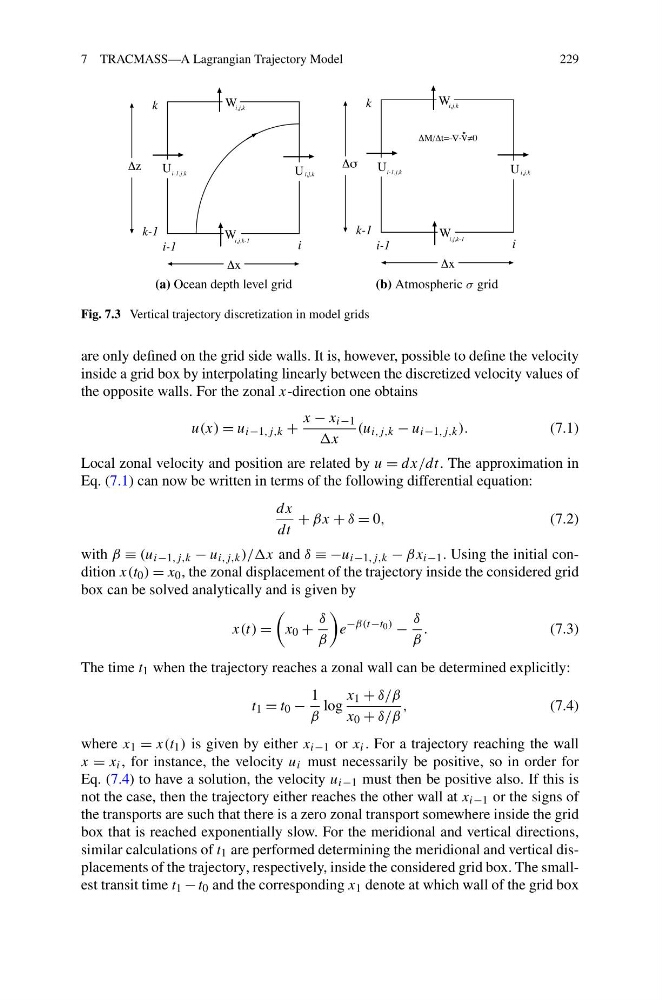
Fig. 7.3 Vertical trajectory discretization in model grids
are only defined on the grid side walls. It is, however, possible to define the velocity
inside a grid box by interpolating linearly between the discretized velocity values of
the opposite walls. For the zonal x-direction one obtains
u(x) = u i−1,j,k +
x − x i−1
x
(u i,j,k − u i−1,j,k ).
(7.1)
Local zonal velocity and position are related by u = dx/dt. The approximation in
Eq. (7.1) can now be written in terms of the following differential equation:
dx
dt
+ βx + δ = 0,
(7.2)
with β ≡ (u i−1,j,k − u i,j,k )//x and δ ≡ −u i−1,j,k − βx i−1 . Using the initial condition x(t 0 ) = x 0 , the zonal displacement of the trajectory inside the considered grid
box can be solved analytically and is given by
x(t) =
x 0 +
δ
β
e
−β(t−t 0 )
−
δ
β
.
(7.3)
The time t 1 when the trajectory reaches a zonal wall can be determined explicitly:
t 1 = t 0 −
1
β
log
x 1 + δ/β
x 0 + δ/β
,
(7.4)
where x 1 = x(t 1 ) is given by either x i−1 or x i . For a trajectory reaching the wall
x = x i , for instance, the velocity u i must necessarily be positive, so in order for
Eq. (7.4) to have a solution, the velocity u i−1 must then be positive also. If this is
not the case, then the trajectory either reaches the other wall at x i−1 or the signs of
the transports are such that there is a zero zonal transport somewhere inside the grid
box that is reached exponentially slow. For the meridional and vertical directions,
similar calculations of t 1 are performed determining the meridional and vertical displacements of the trajectory, respectively, inside the considered grid box. The smallest transit time t 1 − t 0 and the corresponding x 1 denote at which wall of the grid box
229
Fig. 7.3 Vertical trajectory discretization in model grids
are only defined on the grid side walls. It is, however, possible to define the velocity
inside a grid box by interpolating linearly between the discretized velocity values of
the opposite walls. For the zonal x-direction one obtains
u(x) = u i−1,j,k +
x − x i−1
x
(u i,j,k − u i−1,j,k ).
(7.1)
Local zonal velocity and position are related by u = dx/dt. The approximation in
Eq. (7.1) can now be written in terms of the following differential equation:
dx
dt
+ βx + δ = 0,
(7.2)
with β ≡ (u i−1,j,k − u i,j,k )//x and δ ≡ −u i−1,j,k − βx i−1 . Using the initial condition x(t 0 ) = x 0 , the zonal displacement of the trajectory inside the considered grid
box can be solved analytically and is given by
x(t) =
x 0 +
δ
β
e
−β(t−t 0 )
−
δ
β
.
(7.3)
The time t 1 when the trajectory reaches a zonal wall can be determined explicitly:
t 1 = t 0 −
1
β
log
x 1 + δ/β
x 0 + δ/β
,
(7.4)
where x 1 = x(t 1 ) is given by either x i−1 or x i . For a trajectory reaching the wall
x = x i , for instance, the velocity u i must necessarily be positive, so in order for
Eq. (7.4) to have a solution, the velocity u i−1 must then be positive also. If this is
not the case, then the trajectory either reaches the other wall at x i−1 or the signs of
the transports are such that there is a zero zonal transport somewhere inside the grid
box that is reached exponentially slow. For the meridional and vertical directions,
similar calculations of t 1 are performed determining the meridional and vertical displacements of the trajectory, respectively, inside the considered grid box. The smallest transit time t 1 − t 0 and the corresponding x 1 denote at which wall of the grid box