

228
K. Döös et al.
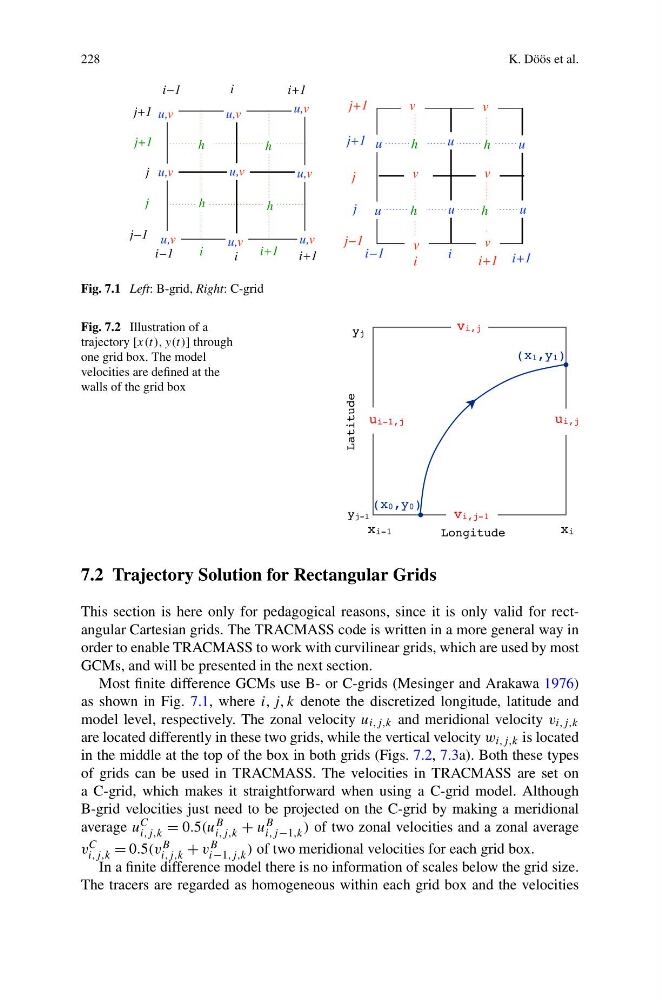
Fig. 7.1 Left: B-grid, Right: C-grid
Fig. 7.2 Illustration of a
trajectory [x(t), y(t)] through
one grid box. The model
velocities are defined at the
walls of the grid box
7.2 Trajectory Solution for Rectangular Grids
This section is here only for pedagogical reasons, since it is only valid for rectangular Cartesian grids. The TRACMASS code is written in a more general way in
order to enable TRACMASS to work with curvilinear grids, which are used by most
GCMs, and will be presented in the next section.
Most finite difference GCMs use B- or C-grids (Mesinger and Arakawa 1976)
as shown in Fig. 7.1, where i, j, k denote the discretized longitude, latitude and
model level, respectively. The zonal velocity u i,j,k and meridional velocity v i,j,k
are located differently in these two grids, while the vertical velocity w i,j,k is located
in the middle at the top of the box in both grids (Figs. 7.2, 7.3a). Both these types
of grids can be used in TRACMASS. The velocities in TRACMASS are set on
a C-grid, which makes it straightforward when using a C-grid model. Although
B-grid velocities just need to be projected on the C-grid by making a meridional
average u C
i,j,k = 0.5(u B
i,j,k + u B
i,j −1,k ) of two zonal velocities and a zonal average
v C
i,j,k = 0.5(v B
i,j,k + v B
i−1,j,k ) of two meridional velocities for each grid box.
In a finite difference model there is no information of scales below the grid size.
The tracers are regarded as homogeneous within each grid box and the velocities
K. Döös et al.
Fig. 7.1 Left: B-grid, Right: C-grid
Fig. 7.2 Illustration of a
trajectory [x(t), y(t)] through
one grid box. The model
velocities are defined at the
walls of the grid box
7.2 Trajectory Solution for Rectangular Grids
This section is here only for pedagogical reasons, since it is only valid for rectangular Cartesian grids. The TRACMASS code is written in a more general way in
order to enable TRACMASS to work with curvilinear grids, which are used by most
GCMs, and will be presented in the next section.
Most finite difference GCMs use B- or C-grids (Mesinger and Arakawa 1976)
as shown in Fig. 7.1, where i, j, k denote the discretized longitude, latitude and
model level, respectively. The zonal velocity u i,j,k and meridional velocity v i,j,k
are located differently in these two grids, while the vertical velocity w i,j,k is located
in the middle at the top of the box in both grids (Figs. 7.2, 7.3a). Both these types
of grids can be used in TRACMASS. The velocities in TRACMASS are set on
a C-grid, which makes it straightforward when using a C-grid model. Although
B-grid velocities just need to be projected on the C-grid by making a meridional
average u C
i,j,k = 0.5(u B
i,j,k + u B
i,j −1,k ) of two zonal velocities and a zonal average
v C
i,j,k = 0.5(v B
i,j,k + v B
i−1,j,k ) of two meridional velocities for each grid box.
In a finite difference model there is no information of scales below the grid size.
The tracers are regarded as homogeneous within each grid box and the velocities