

Vorticity
77
4.3. Potential vorticity
It is now time to introduce the important concept of potential vorticity. In
many flows there are constraints of the motion of fluid parcels set by particular
invariants. In non-rotating flows Kelvin’s theorem is one of these constraints.
These constraints become more powerful when they hold for scalar quantities
instead of for vector quantities. Potential vorticity is one of these scalar quantities
and we will introduce the concept below in its most general form.
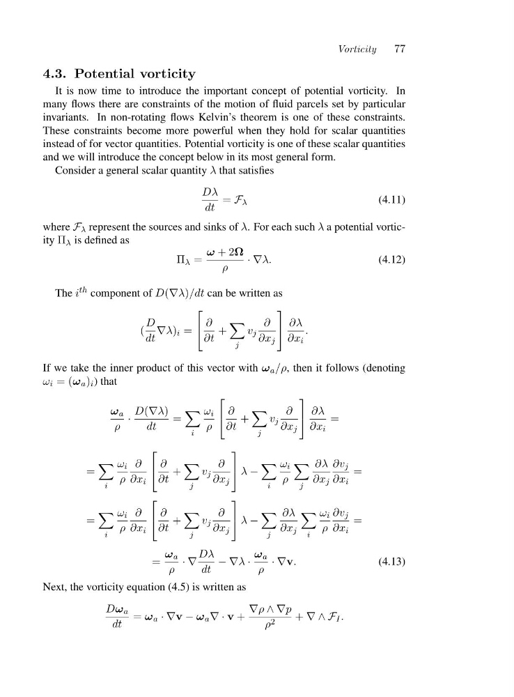
Consider a general scalar quantity λ that satisfies
Dλ
dt
= F λ
(4.11)
where F λ represent the sources and sinks of λ. For each such λ a potential vorticity Π λ is defined as
Π λ =
ω +2Ω
ρ
·∇λ.
(4.12)
The i th component of D(∇λ)/dt can be written as
(
D
dt
∇λ) i =
⎡
⎣ ∂
∂t
+
j
v j
∂
∂x j
⎤
⎦ ∂λ
∂x i
.
If we take the inner product of this vector with ω a /ρ, then it follows (denoting
ω i =(ω a ) i )that
ω a
ρ
·
D(∇λ)
dt
=
i
ω i
ρ
⎡
⎣ ∂
∂t
+
j
v j
∂
∂x j
⎤
⎦ ∂λ
∂x i
=
=
i
ω i
ρ
∂
∂x i
⎡
⎣ ∂
∂t
+
j
v j
∂
∂x j
⎤
⎦ λ −
i
ω i
ρ
j
∂λ
∂x j
∂v j
∂x i
=
=
i
ω i
ρ
∂
∂x i
⎡
⎣ ∂
∂t
+
j
v j
∂
∂x j
⎤
⎦ λ −
j
∂λ
∂x j
i
ω i
ρ
∂v j
∂x i
=
=
ω a
ρ
·∇
Dλ
dt
−∇λ ·
ω a
ρ
·∇v.
(4.13)
Next, the vorticity equation (4.5) is written as
Dω a
dt
= ω a ·∇v − ω a ∇·v +
∇ρ ∧∇p
ρ 2
+ ∇∧F I .
77
4.3. Potential vorticity
It is now time to introduce the important concept of potential vorticity. In
many flows there are constraints of the motion of fluid parcels set by particular
invariants. In non-rotating flows Kelvin’s theorem is one of these constraints.
These constraints become more powerful when they hold for scalar quantities
instead of for vector quantities. Potential vorticity is one of these scalar quantities
and we will introduce the concept below in its most general form.
Consider a general scalar quantity λ that satisfies
Dλ
dt
= F λ
(4.11)
where F λ represent the sources and sinks of λ. For each such λ a potential vorticity Π λ is defined as
Π λ =
ω +2Ω
ρ
·∇λ.
(4.12)
The i th component of D(∇λ)/dt can be written as
(
D
dt
∇λ) i =
⎡
⎣ ∂
∂t
+
j
v j
∂
∂x j
⎤
⎦ ∂λ
∂x i
.
If we take the inner product of this vector with ω a /ρ, then it follows (denoting
ω i =(ω a ) i )that
ω a
ρ
·
D(∇λ)
dt
=
i
ω i
ρ
⎡
⎣ ∂
∂t
+
j
v j
∂
∂x j
⎤
⎦ ∂λ
∂x i
=
=
i
ω i
ρ
∂
∂x i
⎡
⎣ ∂
∂t
+
j
v j
∂
∂x j
⎤
⎦ λ −
i
ω i
ρ
j
∂λ
∂x j
∂v j
∂x i
=
=
i
ω i
ρ
∂
∂x i
⎡
⎣ ∂
∂t
+
j
v j
∂
∂x j
⎤
⎦ λ −
j
∂λ
∂x j
i
ω i
ρ
∂v j
∂x i
=
=
ω a
ρ
·∇
Dλ
dt
−∇λ ·
ω a
ρ
·∇v.
(4.13)
Next, the vorticity equation (4.5) is written as
Dω a
dt
= ω a ·∇v − ω a ∇·v +
∇ρ ∧∇p
ρ 2
+ ∇∧F I .