

76
DYNAMICAL OCEANOGRAPHY
4.2.3. Diffusion of vorticity
Consider a flow of a viscous liquid with (in Cartesian coordinates) F I = ν ∇ 2 v,
where ν is the kinematic viscosity. If we take the rotation of this term (as it
appears in the vorticity equation (4.5)), it follows that ∇∧F I = ν ∇ 2 ω.I m a g -
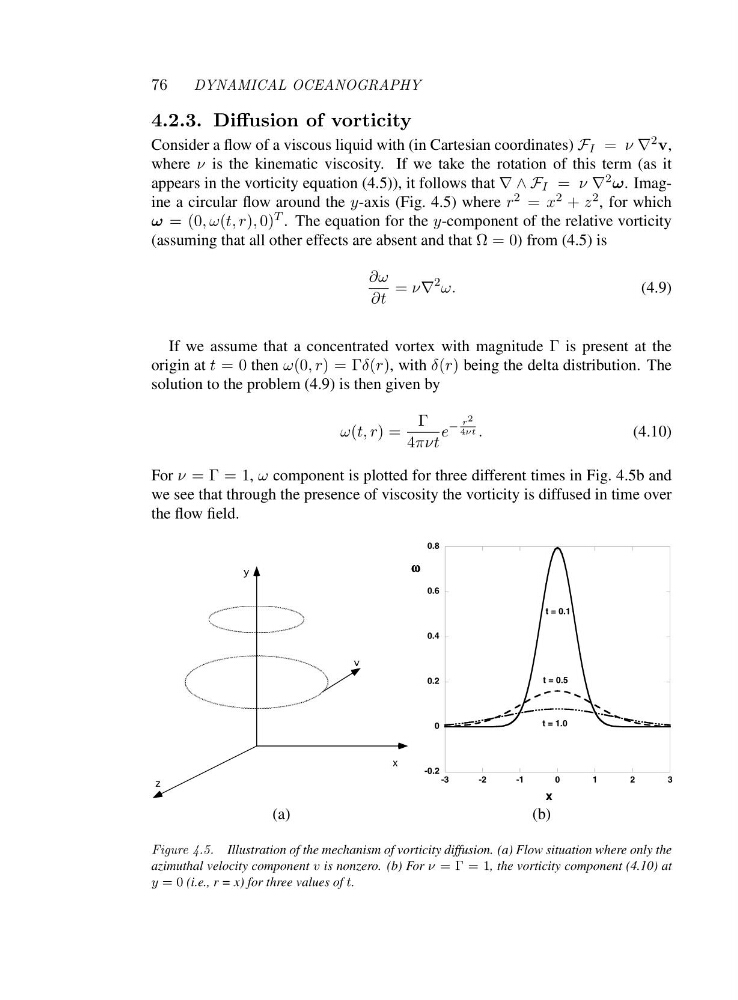
ine a circular flow around the y-axis (Fig. 4.5) where r 2 = x 2 + z 2 , for which
ω =( 0 ,ω(t, r), 0) T . The equation for the y-component of the relative vorticity
(assuming that all other effects are absent and that Ω=0) from (4.5) is
∂ω
∂t
= ν∇
2 ω.
(4.9)
If we assume that a concentrated vortex with magnitude Γ is present at the
origin at t =0then ω(0,r)=Γ δ(r), with δ(r) being the delta distribution. The
solution to the problem (4.9) is then given by
ω(t, r)=
Γ
4πνt
e
−
r 2
4νt .
(4.10)
For ν =Γ=1 , ω component is plotted for three different times in Fig. 4.5b and
we see that through the presence of viscosity the vorticity is diffused in time over
the flow field.
(a)
-0.2
0
0.2
0.4
0.6
0.8
- 3
- 2
- 10123
ω ω ω
ω
x
t = 0.1
t = 0.5
t = 1.0
(b)
Figure 4.5. Illustration of the mechanism of vorticity diffusion. (a) Flow situation where only the
azimuthal velocity component v is nonzero. (b) For ν =Γ=1 , the vorticity component (4.10) at
y =0(i.e., r = x) for three values of t.
DYNAMICAL OCEANOGRAPHY
4.2.3. Diffusion of vorticity
Consider a flow of a viscous liquid with (in Cartesian coordinates) F I = ν ∇ 2 v,
where ν is the kinematic viscosity. If we take the rotation of this term (as it
appears in the vorticity equation (4.5)), it follows that ∇∧F I = ν ∇ 2 ω.I m a g -
ine a circular flow around the y-axis (Fig. 4.5) where r 2 = x 2 + z 2 , for which
ω =( 0 ,ω(t, r), 0) T . The equation for the y-component of the relative vorticity
(assuming that all other effects are absent and that Ω=0) from (4.5) is
∂ω
∂t
= ν∇
2 ω.
(4.9)
If we assume that a concentrated vortex with magnitude Γ is present at the
origin at t =0then ω(0,r)=Γ δ(r), with δ(r) being the delta distribution. The
solution to the problem (4.9) is then given by
ω(t, r)=
Γ
4πνt
e
−
r 2
4νt .
(4.10)
For ν =Γ=1 , ω component is plotted for three different times in Fig. 4.5b and
we see that through the presence of viscosity the vorticity is diffused in time over
the flow field.
(a)
-0.2
0
0.2
0.4
0.6
0.8
- 3
- 2
- 10123
ω ω ω
ω
x
t = 0.1
t = 0.5
t = 1.0
(b)
Figure 4.5. Illustration of the mechanism of vorticity diffusion. (a) Flow situation where only the
azimuthal velocity component v is nonzero. (b) For ν =Γ=1 , the vorticity component (4.10) at
y =0(i.e., r = x) for three values of t.