

Thermohaline circulation
389
anomalies. The atmosphere exerts quite a strong control on the sea surface temperature anomalies, but salinity in the ocean does not affect the freshwater flux
at all. In the two-box model in section 15.3, these different response time scales
of salinity and temperature, with τ S =1 /R S and τ T =1 /R T , were taken into
account by the coefficient η 3 = R S /R T = τ T /τ S , which was smaller than unity.
In general, the different surface boundary conditions for temperature and salinity
are referred to as mixed boundary conditions. The extreme case is a prescribed
surface temperature (τ T << 1) and prescribed surface freshwater flux (τ S >> 1)
for which surface temperature perturbations are essentially zero.
Together, the advective feedback and the different response time scales provide
a potential mechanism of change of the thermohaline circulation. Consider the
thermally driven circulation as in Fig. 16.9 and imagine that a surface freshwater
anomaly is suddenly present in the north part of the domain. Because the density
is lowered in the north, the meridional buoyancy gradient decreases and hence the
strength of the circulation decreases. The effect is that both the northward salt
and heat transport decrease. Now, the negative heat anomaly is rapidly damped
at the sea surface, but the freshwater anomaly is not damped at all and hence
amplifies the original freshwater perturbation. This positive feedback is able to
rapidly weaken the thermally driven overturning circulation.
16.5.2. Convective feedback
A convective feedback may also be responsible for multiple equilibria. In
Fig. 16.10 we consider a box model with time-varying temperature T ∗ and salinity
S ∗ due to a surface heat flux F T = α(T a − T ∗ ) and surface salinity flux F S in the
surface box, coupled to a box with constant temperature T i and S i and constant
prescribed flow rate q. Convective exchange with time constant τ −1 occurs if the
surface water becomes denser than the deep water, which has constant temperature T b and salinity S b .
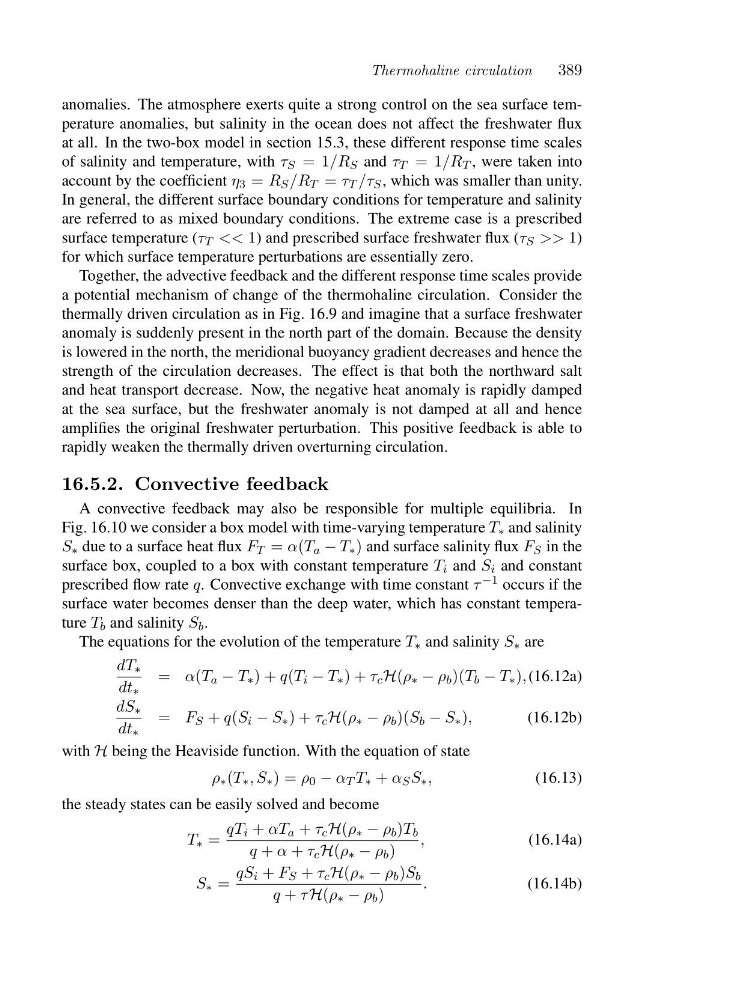
The equations for the evolution of the temperature T ∗ and salinity S ∗ are
dT ∗
dt ∗
= α(T a − T ∗ )+q(T i − T ∗ )+τ c H(ρ ∗ − ρ b )(T b − T ∗ ), (16.12a)
dS ∗
dt ∗
= F S + q(S i − S ∗ )+τ c H(ρ ∗ − ρ b )(S b − S ∗ ),
(16.12b)
with H being the Heaviside function. With the equation of state
ρ ∗ (T ∗ ,S ∗ )=ρ 0 − α T T ∗ + α S S ∗ ,
(16.13)
the steady states can be easily solved and become
T ∗ =
qT i + αT a + τ c H(ρ ∗ − ρ b )T b
q + α + τ c H(ρ ∗ − ρ b )
,
(16.14a)
S ∗ =
qS i + F S + τ c H(ρ ∗ − ρ b )S b
q + τ H(ρ ∗ − ρ b )
.
(16.14b)
389
anomalies. The atmosphere exerts quite a strong control on the sea surface temperature anomalies, but salinity in the ocean does not affect the freshwater flux
at all. In the two-box model in section 15.3, these different response time scales
of salinity and temperature, with τ S =1 /R S and τ T =1 /R T , were taken into
account by the coefficient η 3 = R S /R T = τ T /τ S , which was smaller than unity.
In general, the different surface boundary conditions for temperature and salinity
are referred to as mixed boundary conditions. The extreme case is a prescribed
surface temperature (τ T << 1) and prescribed surface freshwater flux (τ S >> 1)
for which surface temperature perturbations are essentially zero.
Together, the advective feedback and the different response time scales provide
a potential mechanism of change of the thermohaline circulation. Consider the
thermally driven circulation as in Fig. 16.9 and imagine that a surface freshwater
anomaly is suddenly present in the north part of the domain. Because the density
is lowered in the north, the meridional buoyancy gradient decreases and hence the
strength of the circulation decreases. The effect is that both the northward salt
and heat transport decrease. Now, the negative heat anomaly is rapidly damped
at the sea surface, but the freshwater anomaly is not damped at all and hence
amplifies the original freshwater perturbation. This positive feedback is able to
rapidly weaken the thermally driven overturning circulation.
16.5.2. Convective feedback
A convective feedback may also be responsible for multiple equilibria. In
Fig. 16.10 we consider a box model with time-varying temperature T ∗ and salinity
S ∗ due to a surface heat flux F T = α(T a − T ∗ ) and surface salinity flux F S in the
surface box, coupled to a box with constant temperature T i and S i and constant
prescribed flow rate q. Convective exchange with time constant τ −1 occurs if the
surface water becomes denser than the deep water, which has constant temperature T b and salinity S b .
The equations for the evolution of the temperature T ∗ and salinity S ∗ are
dT ∗
dt ∗
= α(T a − T ∗ )+q(T i − T ∗ )+τ c H(ρ ∗ − ρ b )(T b − T ∗ ), (16.12a)
dS ∗
dt ∗
= F S + q(S i − S ∗ )+τ c H(ρ ∗ − ρ b )(S b − S ∗ ),
(16.12b)
with H being the Heaviside function. With the equation of state
ρ ∗ (T ∗ ,S ∗ )=ρ 0 − α T T ∗ + α S S ∗ ,
(16.13)
the steady states can be easily solved and become
T ∗ =
qT i + αT a + τ c H(ρ ∗ − ρ b )T b
q + α + τ c H(ρ ∗ − ρ b )
,
(16.14a)
S ∗ =
qS i + F S + τ c H(ρ ∗ − ρ b )S b
q + τ H(ρ ∗ − ρ b )
.
(16.14b)