

390
DYNAMICAL OCEANOGRAPHY
T
S
T
S
T
S
b
b
i
i
F
F
TS
q
τ c
*
*
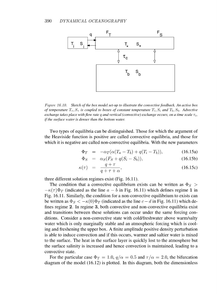
Figure 16.10. Sketch of the box model set-up to illustrate the convective feedback. An active box
of temperature T∗,S∗ is coupled to boxes of constant temperature Ti,Si and Tb,Sb. Advective
exchange takes place with flow rate q and vertical (convective) exchange occurs, on a time scale τc,
if the surface water is denser than the bottom water.
Two types of equilibria can be distinguished. Those for which the argument of
the Heaviside function is positive are called convective equilibria, and those for
which it is negative are called non-convective equilibria. With the new parameters
Φ T = −α T (α(T a − T b )+q(T i − T b )),
(16.15a)
Φ S = α S (F S + q(S i − S b )),
(16.15b)
κ(τ )=
q + τ
q + τ + α
,
(16.15c)
three different solution regimes exist (Fig. 16.11).
The condition that a convective equilibrium exists can be written as Φ S >
−κ(τ )Φ T (indicated as the line a − b in Fig. 16.11) which defines regime 1 in
Fig. 16.11. Similarly, the condition for a non-convective equilibrium to exists can
be written as Φ S < −κ(0)Φ T (indicated as the line c − d in Fig. 16.11) which defines regime 2. In regime 3, both convective and non-convective equilibria exist
and transitions between these solutions can occur under the same forcing conditions. Consider a non-convective state with cold/freshwater above warm/salty
water which is only marginally stable and an atmospheric forcing which is cooling and freshening the upper box. A finite amplitude positive density perturbation
is able to induce convection and if this occurs, warmer and saltier water is mixed
to the surface. The heat in the surface layer is quickly lost to the atmosphere but
the surface salinity is increased and hence convection is maintained, leading to a
convective state.
For the particular case Φ T =1 .0, q/α =0 .5 and τ/α =2 .0, the bifurcation
diagram of the model (16.12) is plotted. In this diagram, both the dimensionless
DYNAMICAL OCEANOGRAPHY
T
S
T
S
T
S
b
b
i
i
F
F
TS
q
τ c
*
*
Figure 16.10. Sketch of the box model set-up to illustrate the convective feedback. An active box
of temperature T∗,S∗ is coupled to boxes of constant temperature Ti,Si and Tb,Sb. Advective
exchange takes place with flow rate q and vertical (convective) exchange occurs, on a time scale τc,
if the surface water is denser than the bottom water.
Two types of equilibria can be distinguished. Those for which the argument of
the Heaviside function is positive are called convective equilibria, and those for
which it is negative are called non-convective equilibria. With the new parameters
Φ T = −α T (α(T a − T b )+q(T i − T b )),
(16.15a)
Φ S = α S (F S + q(S i − S b )),
(16.15b)
κ(τ )=
q + τ
q + τ + α
,
(16.15c)
three different solution regimes exist (Fig. 16.11).
The condition that a convective equilibrium exists can be written as Φ S >
−κ(τ )Φ T (indicated as the line a − b in Fig. 16.11) which defines regime 1 in
Fig. 16.11. Similarly, the condition for a non-convective equilibrium to exists can
be written as Φ S < −κ(0)Φ T (indicated as the line c − d in Fig. 16.11) which defines regime 2. In regime 3, both convective and non-convective equilibria exist
and transitions between these solutions can occur under the same forcing conditions. Consider a non-convective state with cold/freshwater above warm/salty
water which is only marginally stable and an atmospheric forcing which is cooling and freshening the upper box. A finite amplitude positive density perturbation
is able to induce convection and if this occurs, warmer and saltier water is mixed
to the surface. The heat in the surface layer is quickly lost to the atmosphere but
the surface salinity is increased and hence convection is maintained, leading to a
convective state.
For the particular case Φ T =1 .0, q/α =0 .5 and τ/α =2 .0, the bifurcation
diagram of the model (16.12) is plotted. In this diagram, both the dimensionless