

386
DYNAMICAL OCEANOGRAPHY
on the solution branches, indicated by L 1 and L 2 , play a central role in the origin of these equilibria. The regime diagram in Fig. 16.7c provides a complete
overview of where in the parameter plane these multiple equilibria occur.
16.4. Stability of equilibrium solutions
If a particular steady state from the previous section is indicated by (T,S),the
next step is to consider the evolution of perturbations ( ˜
T, ˜
S) on this steady state,
T = T + ˜
T,
(16.7a)
S = S + ˜
S.
(16.7b)
For the box model the notation M is used for a smoothed version of the modulus
function, i.e.
M(Ψ) = [H(Ψ) −H(−Ψ)] Ψ,
where H is a smoothed version of the Heaviside function, for example
H(Ψ) =
1
2
(1 + tanh
Ψ
ǫ
); ǫ ≪ 1,
(16.8)
such that derivatives of M exist. For the linear stability boundary, quadratic interactions in the perturbations are neglected and using
M(Ψ+ ˜
Ψ) = M(Ψ) + M
′ (Ψ) ˜
Ψ+···,
leads to the evolution equations
d ˜
T
dt
= −
(1 + M(Ψ)) ˜
T + M
′ (Ψ)T ( ˜
T − ˜
S)
,
(16.9a)
d ˜
S
dt
= −
(η 3 + M(Ψ)) ˜
S + M
′ (Ψ)S ( ˜
T − ˜
S)
,
(16.9b)
with ˜
Ψ= ˜
T − ˜
S. These equations admit solutions of the form
˜
T = ˆ
Te
σt ; ˜
S = ˆ
Se
σt ,
(16.10)
where σ = σ r + iσ i is the complex growth factor. The real part σ r monitors the
exponential growth rate of the perturbations. Hence, when σ r < 0 for a particular
perturbation ( ˆ
T, ˆ
S) this perturbation is damped and when σ r > 0 it will grow,
leading to instability of the steady state. Substituting these expressions into the
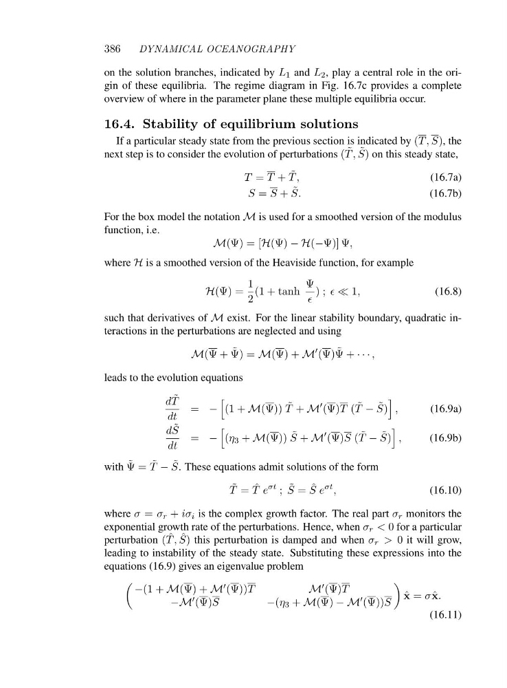
equations (16.9) gives an eigenvalue problem
−(1 + M(Ψ) + M ′ (Ψ))T
M ′ (Ψ)T
−M ′ (Ψ)S
−(η 3 + M(Ψ) −M ′ (Ψ))S
ˆ
x = σˆ x.
(16.11)
DYNAMICAL OCEANOGRAPHY
on the solution branches, indicated by L 1 and L 2 , play a central role in the origin of these equilibria. The regime diagram in Fig. 16.7c provides a complete
overview of where in the parameter plane these multiple equilibria occur.
16.4. Stability of equilibrium solutions
If a particular steady state from the previous section is indicated by (T,S),the
next step is to consider the evolution of perturbations ( ˜
T, ˜
S) on this steady state,
T = T + ˜
T,
(16.7a)
S = S + ˜
S.
(16.7b)
For the box model the notation M is used for a smoothed version of the modulus
function, i.e.
M(Ψ) = [H(Ψ) −H(−Ψ)] Ψ,
where H is a smoothed version of the Heaviside function, for example
H(Ψ) =
1
2
(1 + tanh
Ψ
ǫ
); ǫ ≪ 1,
(16.8)
such that derivatives of M exist. For the linear stability boundary, quadratic interactions in the perturbations are neglected and using
M(Ψ+ ˜
Ψ) = M(Ψ) + M
′ (Ψ) ˜
Ψ+···,
leads to the evolution equations
d ˜
T
dt
= −
(1 + M(Ψ)) ˜
T + M
′ (Ψ)T ( ˜
T − ˜
S)
,
(16.9a)
d ˜
S
dt
= −
(η 3 + M(Ψ)) ˜
S + M
′ (Ψ)S ( ˜
T − ˜
S)
,
(16.9b)
with ˜
Ψ= ˜
T − ˜
S. These equations admit solutions of the form
˜
T = ˆ
Te
σt ; ˜
S = ˆ
Se
σt ,
(16.10)
where σ = σ r + iσ i is the complex growth factor. The real part σ r monitors the
exponential growth rate of the perturbations. Hence, when σ r < 0 for a particular
perturbation ( ˆ
T, ˆ
S) this perturbation is damped and when σ r > 0 it will grow,
leading to instability of the steady state. Substituting these expressions into the
equations (16.9) gives an eigenvalue problem
−(1 + M(Ψ) + M ′ (Ψ))T
M ′ (Ψ)T
−M ′ (Ψ)S
−(η 3 + M(Ψ) −M ′ (Ψ))S
ˆ
x = σˆ x.
(16.11)