

Thermohaline circulation
385
-0.5
0
0.5
1
1.5
2
0
0.5
1
1.5
2
η η
η
η 2
T, S
T
S
TH
SA
(a)
-0.5
0
0.5
1
1.5
2
2.5
3
3.5
0
0.5
1
1.5
2
η η
η
η 2
T, S
S
T
L 1
L 2
(b)
0
0.5
1
1.5
2
012345
η η
η
η 2
η η
η
η 1
L 1
L 2
Q
TH
TH + SA
SA
(c)
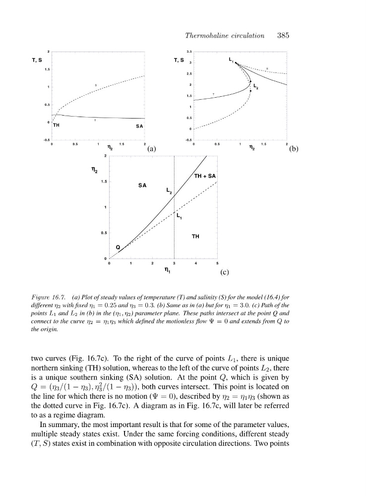
Figure 16.7. (a) Plot of steady values of temperature (T) and salinity (S) for the model (16.4) for
different η2 with fixed η1 =0.25 and η3 =0.3. (b) Same as in (a) but for η1 =3.0. (c) Path of the
points L1 and L2 in (b) in the (η1,η2) parameter plane. These paths intersect at the point Q and
connect to the curve η2 = η1η3 which defined the motionless flow Ψ=0and extends from Q to
the origin.
two curves (Fig. 16.7c). To the right of the curve of points L 1 , there is unique
northern sinking (TH) solution, whereas to the left of the curve of points L 2 ,there
is a unique southern sinking (SA) solution. At the point Q, which is given by
Q =( η 3 /(1 − η 3 ),η 2
3 /(1 − η 3 )), both curves intersect. This point is located on
the line for which there is no motion (Ψ=0), described by η 2 = η 1 η 3 (shown as
the dotted curve in Fig. 16.7c). A diagram as in Fig. 16.7c, will later be referred
to as a regime diagram.
In summary, the most important result is that for some of the parameter values,
multiple steady states exist. Under the same forcing conditions, different steady
(T,S) states exist in combination with opposite circulation directions. Two points
385
-0.5
0
0.5
1
1.5
2
0
0.5
1
1.5
2
η η
η
η 2
T, S
T
S
TH
SA
(a)
-0.5
0
0.5
1
1.5
2
2.5
3
3.5
0
0.5
1
1.5
2
η η
η
η 2
T, S
S
T
L 1
L 2
(b)
0
0.5
1
1.5
2
012345
η η
η
η 2
η η
η
η 1
L 1
L 2
Q
TH
TH + SA
SA
(c)
Figure 16.7. (a) Plot of steady values of temperature (T) and salinity (S) for the model (16.4) for
different η2 with fixed η1 =0.25 and η3 =0.3. (b) Same as in (a) but for η1 =3.0. (c) Path of the
points L1 and L2 in (b) in the (η1,η2) parameter plane. These paths intersect at the point Q and
connect to the curve η2 = η1η3 which defined the motionless flow Ψ=0and extends from Q to
the origin.
two curves (Fig. 16.7c). To the right of the curve of points L 1 , there is unique
northern sinking (TH) solution, whereas to the left of the curve of points L 2 ,there
is a unique southern sinking (SA) solution. At the point Q, which is given by
Q =( η 3 /(1 − η 3 ),η 2
3 /(1 − η 3 )), both curves intersect. This point is located on
the line for which there is no motion (Ψ=0), described by η 2 = η 1 η 3 (shown as
the dotted curve in Fig. 16.7c). A diagram as in Fig. 16.7c, will later be referred
to as a regime diagram.
In summary, the most important result is that for some of the parameter values,
multiple steady states exist. Under the same forcing conditions, different steady
(T,S) states exist in combination with opposite circulation directions. Two points