

Thermohaline circulation
383
the equations (16.5) form a relatively simple mathematical model which immediately suggests proceeding with analytical methods. However, imagine that we
had many more, say ten or more, of these boxes all coupled through exchanges of
heat and salt, which models the horizontal and vertical structure of the exchanges
of these properties in more and more detail. Then, a typical way to proceed would
be to choose parameter values as ‘realistic’ as possible and compute the time
evolution of the temperature and salinity in the boxes, starting from some initial
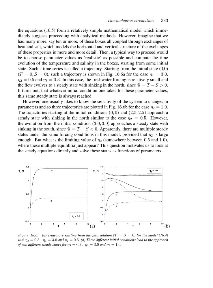
state. Such a time series is called a trajectory. Starting from the initial state (0,0)
(T =0 ,S =0 ), such a trajectory is shown in Fig. 16.6a for the case η 1 =3 .0,
η 2 =0.5 and η 3 =0.3. In this case, the freshwater forcing is relatively small and
the flow evolves to a steady state with sinking in the north, since Ψ=T − S>0.
It turns out, that whatever initial condition one takes for these parameter values,
this same steady state is always reached.
However, one usually likes to know the sensitivity of the system to changes in
parameters and so three trajectories are plotted in Fig. 16.6b for the case η 2 =1.0.
The trajectories starting at the initial conditions (0, 0) and (2.5, 2.5) approach a
steady state with sinking in the north similar to the case η 2 =0 .5.H o w e v e r ,
the evolution from the initial condition (3.0, 3.0) approaches a steady state with
sinking in the south, since Ψ=T − S<0. Apparently, there are multiple steady
states under the same forcing conditions in this model, provided that η 2 is large
enough. But what is the limiting value of η 2 (somewhere between 0.5 and 1.0),
where these multiple equilibria just appear? This question motivates us to look at
the steady equations directly and solve these states as functions of parameters.
-0.5
0
0.5
1
1.5
02468
1 0
T, S
t
T
S
η η η
η 2 = 0.5
(a)
-0.5
0
0.5
1
1.5
2
2.5
3
3.5
02468
1 0
T, S
t
T
S
η η
η
η 2 = 1.0
(b)
Figure 16.6. (a) Trajectory starting from the zero solution (T = S =0 ) for the model (16.4)
with η3 =0.3 ,η 1 =3.0 and η2 =0.5. (b) Three different initial conditions lead to the approach
of two different steady states for η3 =0.3 ,η 1 =3.0 and η2 =1.0.
383
the equations (16.5) form a relatively simple mathematical model which immediately suggests proceeding with analytical methods. However, imagine that we
had many more, say ten or more, of these boxes all coupled through exchanges of
heat and salt, which models the horizontal and vertical structure of the exchanges
of these properties in more and more detail. Then, a typical way to proceed would
be to choose parameter values as ‘realistic’ as possible and compute the time
evolution of the temperature and salinity in the boxes, starting from some initial
state. Such a time series is called a trajectory. Starting from the initial state (0,0)
(T =0 ,S =0 ), such a trajectory is shown in Fig. 16.6a for the case η 1 =3 .0,
η 2 =0.5 and η 3 =0.3. In this case, the freshwater forcing is relatively small and
the flow evolves to a steady state with sinking in the north, since Ψ=T − S>0.
It turns out, that whatever initial condition one takes for these parameter values,
this same steady state is always reached.
However, one usually likes to know the sensitivity of the system to changes in
parameters and so three trajectories are plotted in Fig. 16.6b for the case η 2 =1.0.
The trajectories starting at the initial conditions (0, 0) and (2.5, 2.5) approach a
steady state with sinking in the north similar to the case η 2 =0 .5.H o w e v e r ,
the evolution from the initial condition (3.0, 3.0) approaches a steady state with
sinking in the south, since Ψ=T − S<0. Apparently, there are multiple steady
states under the same forcing conditions in this model, provided that η 2 is large
enough. But what is the limiting value of η 2 (somewhere between 0.5 and 1.0),
where these multiple equilibria just appear? This question motivates us to look at
the steady equations directly and solve these states as functions of parameters.
-0.5
0
0.5
1
1.5
02468
1 0
T, S
t
T
S
η η η
η 2 = 0.5
(a)
-0.5
0
0.5
1
1.5
2
2.5
3
3.5
02468
1 0
T, S
t
T
S
η η
η
η 2 = 1.0
(b)
Figure 16.6. (a) Trajectory starting from the zero solution (T = S =0 ) for the model (16.4)
with η3 =0.3 ,η 1 =3.0 and η2 =0.5. (b) Three different initial conditions lead to the approach
of two different steady states for η3 =0.3 ,η 1 =3.0 and η2 =1.0.