

382
DYNAMICAL OCEANOGRAPHY
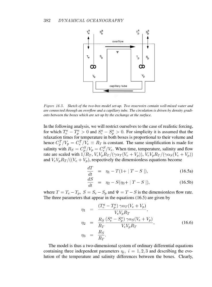
Figure 16.5. Sketch of the two-box model set-up. Two reservoirs contain well-mixed water and
are connected through an overflow and a capillary tube. The circulation is driven by density gradients between the boxes which are set-up by the exchange at the surface.
In the following analysis, we will restrict ourselves to the case of realistic forcing,
for which T a
e − T a
p > 0 and S a
e − S a
p > 0. For simplicity it is assumed that the
relaxation times for temperature in both boxes is proportional to their volume and
hence C T
p /V p = C T
e /V e ≡ R T is constant. The same simplification is made for
salinity with R S = C S
p /V p = C S
e /V e . When time, temperature, salinity and flow
rate are scaled with 1/R T , V e V p R T /(γα T (V e + V p )), V e V p R T /(γα S (V e + V p ))
and V e V p R T /((V e + V p ), respectively the dimensionless equations become
dT
dt
= η 1 − T (1+ | T − S |),
(16.5a)
dS
dt
= η 2 − S(η 3 + | T − S |),
(16.5b)
where T = T e − T p ,S= S e − S p and Ψ=T − S is the dimensionless flow rate.
The three parameters that appear in the equations (16.5) are given by
η 1 =
(T a
e − T a
p ) γα T (V e + V p )
V e V p R T
,
η 2 =
R S
R T
(S a
e − S a
p ) γα S (V e + V p )
V e V p R T
,
(16.6)
η 3 =
R S
R T
.
The model is thus a two-dimensional system of ordinary differential equations
containing three independent parameters η i ,i=1 , 2, 3 and describing the evolution of the temperature and salinity differences between the boxes. Clearly,
DYNAMICAL OCEANOGRAPHY
Figure 16.5. Sketch of the two-box model set-up. Two reservoirs contain well-mixed water and
are connected through an overflow and a capillary tube. The circulation is driven by density gradients between the boxes which are set-up by the exchange at the surface.
In the following analysis, we will restrict ourselves to the case of realistic forcing,
for which T a
e − T a
p > 0 and S a
e − S a
p > 0. For simplicity it is assumed that the
relaxation times for temperature in both boxes is proportional to their volume and
hence C T
p /V p = C T
e /V e ≡ R T is constant. The same simplification is made for
salinity with R S = C S
p /V p = C S
e /V e . When time, temperature, salinity and flow
rate are scaled with 1/R T , V e V p R T /(γα T (V e + V p )), V e V p R T /(γα S (V e + V p ))
and V e V p R T /((V e + V p ), respectively the dimensionless equations become
dT
dt
= η 1 − T (1+ | T − S |),
(16.5a)
dS
dt
= η 2 − S(η 3 + | T − S |),
(16.5b)
where T = T e − T p ,S= S e − S p and Ψ=T − S is the dimensionless flow rate.
The three parameters that appear in the equations (16.5) are given by
η 1 =
(T a
e − T a
p ) γα T (V e + V p )
V e V p R T
,
η 2 =
R S
R T
(S a
e − S a
p ) γα S (V e + V p )
V e V p R T
,
(16.6)
η 3 =
R S
R T
.
The model is thus a two-dimensional system of ordinary differential equations
containing three independent parameters η i ,i=1 , 2, 3 and describing the evolution of the temperature and salinity differences between the boxes. Clearly,