

368
DYNAMICAL OCEANOGRAPHY
where r 2 =(x − x 0 ) 2 +(y − y 0 ) 2 and H 1 and H 0 are constants. Hence, at r =0,
we have H =(H 0 + H 1 ) mandforr ≫ L,wehaveH ≈ H 1 m. We assume that
the right hand side, say F , of (15.44) is known as
F (x, y)=F 0 (
x
x 0
)
2 ,
(15.47)
which is constant in y and increasing quadratically in x. Let us assume that the
Coriolis parameter f is constant. Certainly, the geostrophic contours f/H are
closed. Let furthermore the bottom stress be parameterized as
τ b = ρ 0 R v b ,
(15.48)
with R being constant, then (15.44) becomes
−v b ·∇H +
R
f
∇∧v b = F →−
1
ρ 0 f
J(ψ b ,H)+
R
ρ 0 f 2 ∇
2 ψ b = F, (15.49)
where J is again the Jacobian. For given H and F this is a linear equation for the
streamfunction ψ b which can be solved numerically.
Ex. 15.5
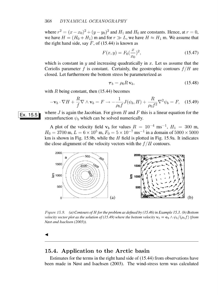
A plot of the velocity field v b for values R =1 0 −4 ms −1 , H 1 = 300 m,
H 0 = 3700 m, L =6× 10 5 m, F 0 =5× 10 −7 ms −1 in a domain of 5000 × 5000
km is shown in Fig. 15.9b, while the H field is plotted in Fig. 15.9a. It indicates
the close alignment of the velocity vectors with the f/H contours.
(a)
(b)
Figure 15.9. (a) Contours of H for the problem as defined by (15.46) in Example 15.3. (b) Bottom
velocity vector plot as the solution of (15.49) where the bottom velocity vb = e3 ∧ ψb/(ρ0f ) (from
Nøst and Isachsen (2003)).
◭
15.4. Application to the Arctic basin
Estimates for the terms in the right hand side of (15.44) from observations have
been made in Nøst and Isachsen (2003). The wind-stress term was calculated
DYNAMICAL OCEANOGRAPHY
where r 2 =(x − x 0 ) 2 +(y − y 0 ) 2 and H 1 and H 0 are constants. Hence, at r =0,
we have H =(H 0 + H 1 ) mandforr ≫ L,wehaveH ≈ H 1 m. We assume that
the right hand side, say F , of (15.44) is known as
F (x, y)=F 0 (
x
x 0
)
2 ,
(15.47)
which is constant in y and increasing quadratically in x. Let us assume that the
Coriolis parameter f is constant. Certainly, the geostrophic contours f/H are
closed. Let furthermore the bottom stress be parameterized as
τ b = ρ 0 R v b ,
(15.48)
with R being constant, then (15.44) becomes
−v b ·∇H +
R
f
∇∧v b = F →−
1
ρ 0 f
J(ψ b ,H)+
R
ρ 0 f 2 ∇
2 ψ b = F, (15.49)
where J is again the Jacobian. For given H and F this is a linear equation for the
streamfunction ψ b which can be solved numerically.
Ex. 15.5
A plot of the velocity field v b for values R =1 0 −4 ms −1 , H 1 = 300 m,
H 0 = 3700 m, L =6× 10 5 m, F 0 =5× 10 −7 ms −1 in a domain of 5000 × 5000
km is shown in Fig. 15.9b, while the H field is plotted in Fig. 15.9a. It indicates
the close alignment of the velocity vectors with the f/H contours.
(a)
(b)
Figure 15.9. (a) Contours of H for the problem as defined by (15.46) in Example 15.3. (b) Bottom
velocity vector plot as the solution of (15.49) where the bottom velocity vb = e3 ∧ ψb/(ρ0f ) (from
Nøst and Isachsen (2003)).
◭
15.4. Application to the Arctic basin
Estimates for the terms in the right hand side of (15.44) from observations have
been made in Nøst and Isachsen (2003). The wind-stress term was calculated