

Arctic Ocean Circulation
367
we evaluate
∇·v g = e 3 ∧∇p ·∇(
1
f
)=−
1
f
v g ·∇f,
(15.40a)
∇·v b = e 3 ∧∇p ·∇(
1
f
)=−
1
f
v b ·∇f,
(15.40b)
and
∇·(Hv b )=∇·(
H
ρ 0 f
e 3 ∧∇p b )=f v b ·∇(
H
f
)=−
H 2
f
v b ·∇(
f
H
). (15.41)
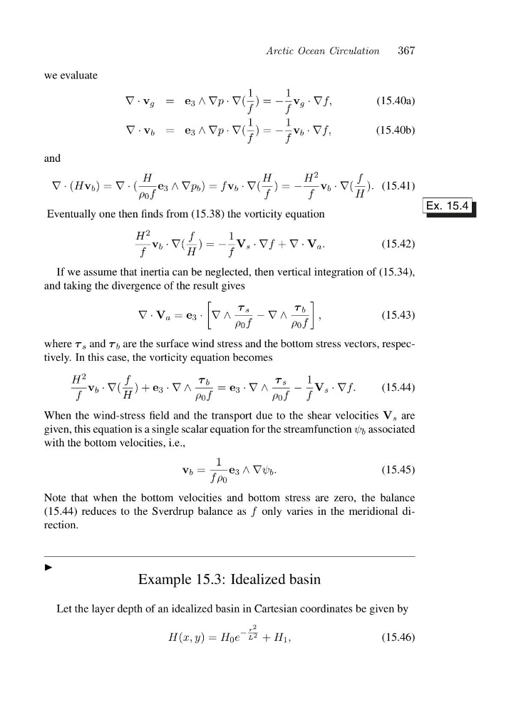
Eventually one then finds from (15.38) the vorticity equation
Ex. 15.4
H 2
f
v b ·∇(
f
H
)=−
1
f
V s ·∇f + ∇·V a .
(15.42)
If we assume that inertia can be neglected, then vertical integration of (15.34),
and taking the divergence of the result gives
∇·V a = e 3 ·
∇∧
τ s
ρ 0 f
−∇∧
τ b
ρ 0 f
,
(15.43)
where τ s and τ b are the surface wind stress and the bottom stress vectors, respectively. In this case, the vorticity equation becomes
H 2
f
v b ·∇(
f
H
)+e 3 ·∇∧
τ b
ρ 0 f
= e 3 ·∇∧
τ s
ρ 0 f
−
1
f
V s ·∇f.
(15.44)
When the wind-stress field and the transport due to the shear velocities V s are
given, this equation is a single scalar equation for the streamfunction ψ b associated
with the bottom velocities, i.e.,
v b =
1
fρ 0
e 3 ∧∇ψ b .
(15.45)
Note that when the bottom velocities and bottom stress are zero, the balance
(15.44) reduces to the Sverdrup balance as f only varies in the meridional direction.
◮
Example 15.3: Idealized basin
Let the layer depth of an idealized basin in Cartesian coordinates be given by
H(x, y)=H 0 e
−
r 2
L 2 + H 1 ,
(15.46)
367
we evaluate
∇·v g = e 3 ∧∇p ·∇(
1
f
)=−
1
f
v g ·∇f,
(15.40a)
∇·v b = e 3 ∧∇p ·∇(
1
f
)=−
1
f
v b ·∇f,
(15.40b)
and
∇·(Hv b )=∇·(
H
ρ 0 f
e 3 ∧∇p b )=f v b ·∇(
H
f
)=−
H 2
f
v b ·∇(
f
H
). (15.41)
Eventually one then finds from (15.38) the vorticity equation
Ex. 15.4
H 2
f
v b ·∇(
f
H
)=−
1
f
V s ·∇f + ∇·V a .
(15.42)
If we assume that inertia can be neglected, then vertical integration of (15.34),
and taking the divergence of the result gives
∇·V a = e 3 ·
∇∧
τ s
ρ 0 f
−∇∧
τ b
ρ 0 f
,
(15.43)
where τ s and τ b are the surface wind stress and the bottom stress vectors, respectively. In this case, the vorticity equation becomes
H 2
f
v b ·∇(
f
H
)+e 3 ·∇∧
τ b
ρ 0 f
= e 3 ·∇∧
τ s
ρ 0 f
−
1
f
V s ·∇f.
(15.44)
When the wind-stress field and the transport due to the shear velocities V s are
given, this equation is a single scalar equation for the streamfunction ψ b associated
with the bottom velocities, i.e.,
v b =
1
fρ 0
e 3 ∧∇ψ b .
(15.45)
Note that when the bottom velocities and bottom stress are zero, the balance
(15.44) reduces to the Sverdrup balance as f only varies in the meridional direction.
◮
Example 15.3: Idealized basin
Let the layer depth of an idealized basin in Cartesian coordinates be given by
H(x, y)=H 0 e
−
r 2
L 2 + H 1 ,
(15.46)