

344
DYNAMICAL OCEANOGRAPHY
x 0
x 1
geostrophic
contours
bottom topography
0
y
x
h 0
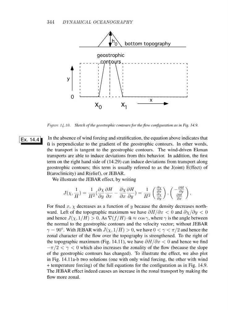
Figure 14.10. Sketch of the geostrophic contours for the flow configuration as in Fig. 14.9.
In the absence of wind forcing and stratification, the equation above indicates that
Ex. 14.4
¯
u is perpendicular to the gradient of the geostrophic contours. In other words,
the transport is tangent to the geostrophic contours. The wind-driven Ekman
transports are able to induce deviations from this behavior. In addition, the first
term on the right hand side of (14.29) can induce deviations from transport along
geostrophic contours; this term is usually referred to as the J(oint) E(ffect) of
B(aroclinicity) and R(elief), or JEBAR.
We illustrate the JEBAR effect, by writing
J(χ,
1
H
)=
1
H 2 (
∂χ
∂y
∂H
∂x
−
∂χ
∂x
∂H
∂y
)=
1
H 2
∂χ
∂x
∂χ
∂y
.
−
∂H
∂y
∂H
∂x
,
For fixed x, χ decreases as a function of y because the density decreases northward. Left of the topographic maximum we have ∂H/∂x < 0 and ∂χ/∂y < 0
and hence J(χ, 1/H) > 0.A s∇(f/H) · ¯
u ≈ cos γ, where γ is the angle between
the normal to the geostrophic contours and the velocity vector; without JEBAR
γ =90 ◦ . With JEBAR with J(χ, 1/H) > 0,wehave0 <γ<π/2 and hence the
zonal character of the flow over the topography is strengthened. To the right of
the topographic maximum (Fig. 14.11), we have ∂H/∂x < 0 and hence we find
−π/2 <γ<0 which also increases the zonality of the flow (because the slope
of the geostrophic contours has changed). To illustrate the effect, we also plot
in Fig. 14.11a-b two solutions (one with only wind forcing, the other with wind
+ temperature forcing) of the full equations for the configuration as in Fig. 14.9.
The JEBAR effect indeed causes an increase in the zonal transport by making the
flow more zonal.
DYNAMICAL OCEANOGRAPHY
x 0
x 1
geostrophic
contours
bottom topography
0
y
x
h 0
Figure 14.10. Sketch of the geostrophic contours for the flow configuration as in Fig. 14.9.
In the absence of wind forcing and stratification, the equation above indicates that
Ex. 14.4
¯
u is perpendicular to the gradient of the geostrophic contours. In other words,
the transport is tangent to the geostrophic contours. The wind-driven Ekman
transports are able to induce deviations from this behavior. In addition, the first
term on the right hand side of (14.29) can induce deviations from transport along
geostrophic contours; this term is usually referred to as the J(oint) E(ffect) of
B(aroclinicity) and R(elief), or JEBAR.
We illustrate the JEBAR effect, by writing
J(χ,
1
H
)=
1
H 2 (
∂χ
∂y
∂H
∂x
−
∂χ
∂x
∂H
∂y
)=
1
H 2
∂χ
∂x
∂χ
∂y
.
−
∂H
∂y
∂H
∂x
,
For fixed x, χ decreases as a function of y because the density decreases northward. Left of the topographic maximum we have ∂H/∂x < 0 and ∂χ/∂y < 0
and hence J(χ, 1/H) > 0.A s∇(f/H) · ¯
u ≈ cos γ, where γ is the angle between
the normal to the geostrophic contours and the velocity vector; without JEBAR
γ =90 ◦ . With JEBAR with J(χ, 1/H) > 0,wehave0 <γ<π/2 and hence the
zonal character of the flow over the topography is strengthened. To the right of
the topographic maximum (Fig. 14.11), we have ∂H/∂x < 0 and hence we find
−π/2 <γ<0 which also increases the zonality of the flow (because the slope
of the geostrophic contours has changed). To illustrate the effect, we also plot
in Fig. 14.11a-b two solutions (one with only wind forcing, the other with wind
+ temperature forcing) of the full equations for the configuration as in Fig. 14.9.
The JEBAR effect indeed causes an increase in the zonal transport by making the
flow more zonal.