

Antarctic Circumpolar Current
343
Ex. 14.3
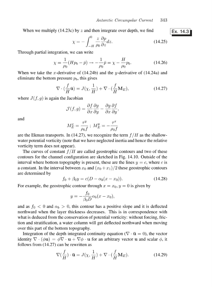
When we multiply (14.23c) by z and then integrate over depth, we find
χ = −
0
−H
z
ρ 0
∂p
∂z
dz.
(14.25)
Through partial integration, we can write
χ =
1
ρ 0
(Hp b − ¯
p) →−
1
ρ 0
¯
p = χ −
H
ρ 0
p b .
(14.26)
When we take the x-derivative of (14.24b) and the y-derivative of (14.24a) and
eliminate the bottom pressure p b ,thisgives
∇·(
f
H
¯
u)=J(χ,
1
H
)+∇·(
f
H
M E ),
(14.27)
where J(f, g) is again the Jacobian
J (f, g)=
∂f
∂x
∂g
∂y
−
∂g
∂x
∂f
∂y
,
and
M
x
E =
τ y
ρ 0 f
; M
y
E = −
τ x
ρ 0 f
are the Ekman transports. In (14.27), we recognize the term f/H as the shallowwater potential vorticity (note that we have neglected inertia and hence the relative
vorticity term does not appear).
The curves of constant f/H are called geostrophic contours and two of these
contours for the channel configuration are sketched in Fig. 14.10. Outside of the
interval where bottom topography is present, these are the lines y = c, where c is
a constant. In the interval between x 0 and (x 0 + x 1 )/2 these geostrophic contours
are determined by
f 0 + β 0 y = c(D − α b (x − x 0 )).
(14.28)
For example, the geostrophic contour through x = x 0 ,y =0is given by
y = −
f 0
β 0 D
α b (x − x 0 ),
and as f 0 < 0 and α b > 0, this contour has a positive slope and it is deflected
northward when the layer thickness decreases. This is in correspondence with
what is deduced from the conservation of potential vorticity: without forcing, friction and stratification, a water column will get deflected northward when moving
over this part of the bottom topography.
Integration of the depth integrated continuity equation (∇·¯ u =0 ), the vector
identity ∇·(φu)=φ∇·u + ∇φ · u for an arbitrary vector u and scalar φ,i t
follows from (14.27) can be rewritten as
∇(
f
H
) · ¯
u = J(χ,
1
H
)+∇·(
f
H
M E ).
(14.29)
343
Ex. 14.3
When we multiply (14.23c) by z and then integrate over depth, we find
χ = −
0
−H
z
ρ 0
∂p
∂z
dz.
(14.25)
Through partial integration, we can write
χ =
1
ρ 0
(Hp b − ¯
p) →−
1
ρ 0
¯
p = χ −
H
ρ 0
p b .
(14.26)
When we take the x-derivative of (14.24b) and the y-derivative of (14.24a) and
eliminate the bottom pressure p b ,thisgives
∇·(
f
H
¯
u)=J(χ,
1
H
)+∇·(
f
H
M E ),
(14.27)
where J(f, g) is again the Jacobian
J (f, g)=
∂f
∂x
∂g
∂y
−
∂g
∂x
∂f
∂y
,
and
M
x
E =
τ y
ρ 0 f
; M
y
E = −
τ x
ρ 0 f
are the Ekman transports. In (14.27), we recognize the term f/H as the shallowwater potential vorticity (note that we have neglected inertia and hence the relative
vorticity term does not appear).
The curves of constant f/H are called geostrophic contours and two of these
contours for the channel configuration are sketched in Fig. 14.10. Outside of the
interval where bottom topography is present, these are the lines y = c, where c is
a constant. In the interval between x 0 and (x 0 + x 1 )/2 these geostrophic contours
are determined by
f 0 + β 0 y = c(D − α b (x − x 0 )).
(14.28)
For example, the geostrophic contour through x = x 0 ,y =0is given by
y = −
f 0
β 0 D
α b (x − x 0 ),
and as f 0 < 0 and α b > 0, this contour has a positive slope and it is deflected
northward when the layer thickness decreases. This is in correspondence with
what is deduced from the conservation of potential vorticity: without forcing, friction and stratification, a water column will get deflected northward when moving
over this part of the bottom topography.
Integration of the depth integrated continuity equation (∇·¯ u =0 ), the vector
identity ∇·(φu)=φ∇·u + ∇φ · u for an arbitrary vector u and scalar φ,i t
follows from (14.27) can be rewritten as
∇(
f
H
) · ¯
u = J(χ,
1
H
)+∇·(
f
H
M E ).
(14.29)