

Antarctic Circumpolar Current
339
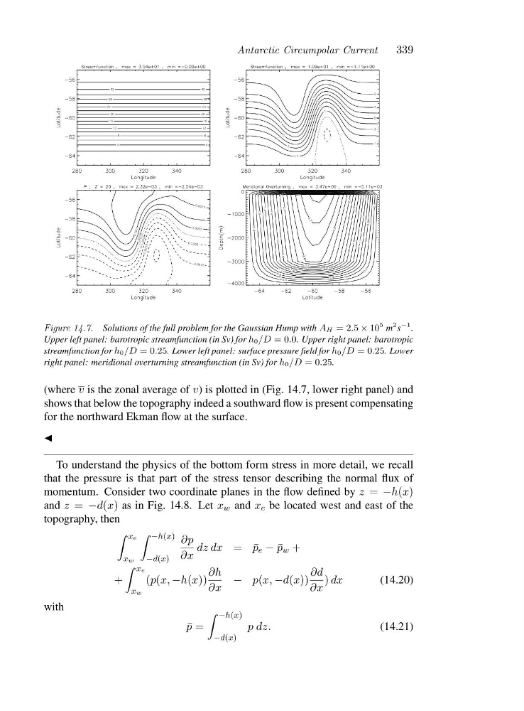
Figure 14.7. Solutions of the full problem for the Gaussian Hump with AH =2.5 × 10
5 m
2 s
−1 .
Upper left panel: barotropic streamfunction (in Sv) for h0/D =0.0. Upper right panel: barotropic
streamfunction for h0/D =0.25. Lower left panel: surface pressure field for h0/D =0.25.Lower
right panel: meridional overturning streamfunction (in Sv) for h0/D =0.25.
(where v is the zonal average of v) is plotted in (Fig. 14.7, lower right panel) and
shows that below the topography indeed a southward flow is present compensating
for the northward Ekman flow at the surface.
◭
To understand the physics of the bottom form stress in more detail, we recall
that the pressure is that part of the stress tensor describing the normal flux of
momentum. Consider two coordinate planes in the flow defined by z = −h(x)
and z = −d(x) as in Fig. 14.8. Let x w and x e be located west and east of the
topography, then
xe
xw
−h(x)
−d(x)
∂p
∂x
dz dx =¯ p e − ¯
p w +
+
xe
xw
(p(x, −h(x))
∂h
∂x
− p(x, −d(x))
∂d
∂x
) dx
(14.20)
with
¯
p =
−h(x)
−d(x)
pdz.
(14.21)
339
Figure 14.7. Solutions of the full problem for the Gaussian Hump with AH =2.5 × 10
5 m
2 s
−1 .
Upper left panel: barotropic streamfunction (in Sv) for h0/D =0.0. Upper right panel: barotropic
streamfunction for h0/D =0.25. Lower left panel: surface pressure field for h0/D =0.25.Lower
right panel: meridional overturning streamfunction (in Sv) for h0/D =0.25.
(where v is the zonal average of v) is plotted in (Fig. 14.7, lower right panel) and
shows that below the topography indeed a southward flow is present compensating
for the northward Ekman flow at the surface.
◭
To understand the physics of the bottom form stress in more detail, we recall
that the pressure is that part of the stress tensor describing the normal flux of
momentum. Consider two coordinate planes in the flow defined by z = −h(x)
and z = −d(x) as in Fig. 14.8. Let x w and x e be located west and east of the
topography, then
xe
xw
−h(x)
−d(x)
∂p
∂x
dz dx =¯ p e − ¯
p w +
+
xe
xw
(p(x, −h(x))
∂h
∂x
− p(x, −d(x))
∂d
∂x
) dx
(14.20)
with
¯
p =
−h(x)
−d(x)
pdz.
(14.21)