338
DYNAMICAL OCEANOGRAPHY
= −
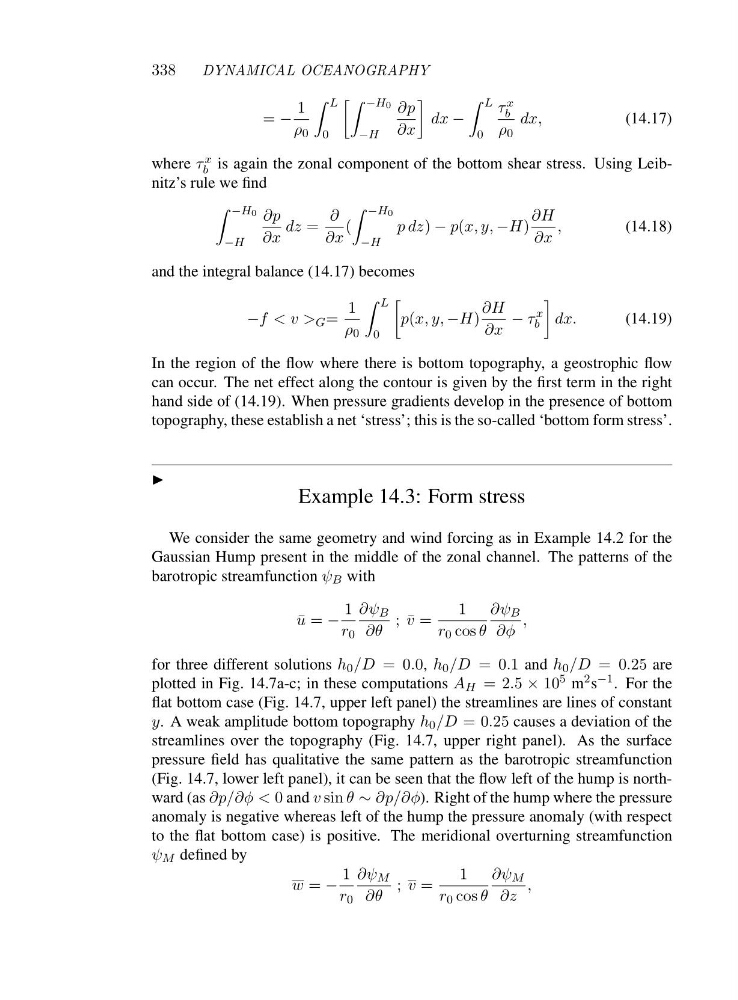
1
ρ 0
L
0
−H0
−H
∂p
∂x
dx −
L
0
τ x
b
ρ 0
dx,
(14.17)
where τ x
b is again the zonal component of the bottom shear stress. Using Leibnitz’s rule we find
−H0
−H
∂p
∂x
dz =
∂
∂x
(
−H0
−H
pdz) − p(x, y, −H)
∂H
∂x
,
(14.18)
and the integral balance (14.17) becomes
−f G =
1
ρ 0
L
0
p(x, y, −H)
∂H
∂x
− τ
x
b
dx.
(14.19)
In the region of the flow where there is bottom topography, a geostrophic flow
can occur. The net effect along the contour is given by the first term in the right
hand side of (14.19). When pressure gradients develop in the presence of bottom
topography, these establish a net ‘stress’; this is the so-called ‘bottom form stress’.
◮
Example 14.3: Form stress
We consider the same geometry and wind forcing as in Example 14.2 for the
Gaussian Hump present in the middle of the zonal channel. The patterns of the
barotropic streamfunction ψ B with
¯
u = −
1
r 0
∂ψ B
∂θ
;¯ v =
1
r 0 cos θ
∂ψ B
∂φ
,
for three different solutions h 0 /D =0 .0, h 0 /D =0 .1 and h 0 /D =0 .25 are
plotted in Fig. 14.7a-c; in these computations A H =2 .5 × 10 5 m 2 s −1 . For the
flat bottom case (Fig. 14.7, upper left panel) the streamlines are lines of constant
y. A weak amplitude bottom topography h 0 /D =0 .25 causes a deviation of the
streamlines over the topography (Fig. 14.7, upper right panel). As the surface
pressure field has qualitative the same pattern as the barotropic streamfunction
(Fig. 14.7, lower left panel), it can be seen that the flow left of the hump is northward (as ∂p/∂φ < 0 and v sin θ ∼ ∂p/∂φ). Right of the hump where the pressure
anomaly is negative whereas left of the hump the pressure anomaly (with respect
to the flat bottom case) is positive. The meridional overturning streamfunction
ψ M defined by
w = −
1
r 0
∂ψ M
∂θ
; v =
1
r 0 cos θ
∂ψ M
∂z
,