

Antarctic Circumpolar Current
335
lateral friction, gives
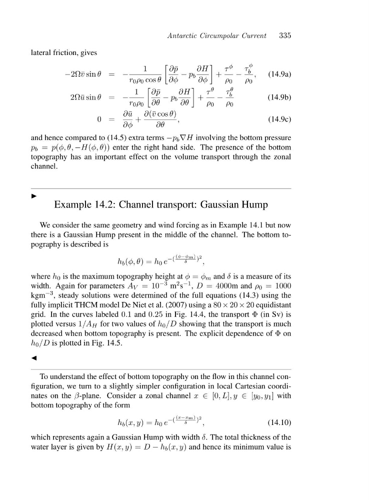
−2Ω¯ v sin θ = −
1
r 0 ρ 0 cos θ
∂ ¯
p
∂φ
− p b
∂H
∂φ
+
τ φ
ρ 0
−
τ
φ
b
ρ 0
,
(14.9a)
2Ω¯ u sin θ = −
1
r 0 ρ 0
∂ ¯
p
∂θ
− p b
∂H
∂θ
+
τ θ
ρ 0
−
τ θ
b
ρ 0
(14.9b)
0=
∂ ¯
u
∂φ
+
∂(¯ v cos θ)
∂θ
,
(14.9c)
and hence compared to (14.5) extra terms −p b ∇H involving the bottom pressure
p b = p(φ, θ, −H(φ, θ)) enter the right hand side. The presence of the bottom
topography has an important effect on the volume transport through the zonal
channel.
◮
Example 14.2: Channel transport: Gaussian Hump
We consider the same geometry and wind forcing as in Example 14.1 but now
there is a Gaussian Hump present in the middle of the channel. The bottom topography is described is
h b (φ, θ)=h 0 e
−(
(φ−φm)
δ
) 2 ,
where h 0 is the maximum topography height at φ = φ m and δ is a measure of its
width. Again for parameters A V =1 0 −3 m 2 s −1 , D = 4000ma n dρ 0 = 1000
kgm −3 , steady solutions were determined of the full equations (14.3) using the
fully implicit THCM model De Niet et al. (2007) using a 80 × 20 × 20 equidistant
grid. In the curves labeled 0.1 and 0.25 in Fig. 14.4, the transport Φ (in Sv) is
plotted versus 1/A H for two values of h 0 /D showing that the transport is much
decreased when bottom topography is present. The explicit dependence of Φ on
h 0 /D is plotted in Fig. 14.5.
◭
To understand the effect of bottom topography on the flow in this channel configuration, we turn to a slightly simpler configuration in local Cartesian coordinates on the β-plane. Consider a zonal channel x ∈ [0,L],y ∈ [y 0 ,y 1 ] with
bottom topography of the form
h b (x, y)=h 0 e
−(
(x−xm)
δ
) 2 ,
(14.10)
which represents again a Gaussian Hump with width δ. The total thickness of the
water layer is given by H(x, y)=D − h b (x, y) and hence its minimum value is
335
lateral friction, gives
−2Ω¯ v sin θ = −
1
r 0 ρ 0 cos θ
∂ ¯
p
∂φ
− p b
∂H
∂φ
+
τ φ
ρ 0
−
τ
φ
b
ρ 0
,
(14.9a)
2Ω¯ u sin θ = −
1
r 0 ρ 0
∂ ¯
p
∂θ
− p b
∂H
∂θ
+
τ θ
ρ 0
−
τ θ
b
ρ 0
(14.9b)
0=
∂ ¯
u
∂φ
+
∂(¯ v cos θ)
∂θ
,
(14.9c)
and hence compared to (14.5) extra terms −p b ∇H involving the bottom pressure
p b = p(φ, θ, −H(φ, θ)) enter the right hand side. The presence of the bottom
topography has an important effect on the volume transport through the zonal
channel.
◮
Example 14.2: Channel transport: Gaussian Hump
We consider the same geometry and wind forcing as in Example 14.1 but now
there is a Gaussian Hump present in the middle of the channel. The bottom topography is described is
h b (φ, θ)=h 0 e
−(
(φ−φm)
δ
) 2 ,
where h 0 is the maximum topography height at φ = φ m and δ is a measure of its
width. Again for parameters A V =1 0 −3 m 2 s −1 , D = 4000ma n dρ 0 = 1000
kgm −3 , steady solutions were determined of the full equations (14.3) using the
fully implicit THCM model De Niet et al. (2007) using a 80 × 20 × 20 equidistant
grid. In the curves labeled 0.1 and 0.25 in Fig. 14.4, the transport Φ (in Sv) is
plotted versus 1/A H for two values of h 0 /D showing that the transport is much
decreased when bottom topography is present. The explicit dependence of Φ on
h 0 /D is plotted in Fig. 14.5.
◭
To understand the effect of bottom topography on the flow in this channel configuration, we turn to a slightly simpler configuration in local Cartesian coordinates on the β-plane. Consider a zonal channel x ∈ [0,L],y ∈ [y 0 ,y 1 ] with
bottom topography of the form
h b (x, y)=h 0 e
−(
(x−xm)
δ
) 2 ,
(14.10)
which represents again a Gaussian Hump with width δ. The total thickness of the
water layer is given by H(x, y)=D − h b (x, y) and hence its minimum value is