

334
DYNAMICAL OCEANOGRAPHY
For parameters A V =1 0 −3 m 2 s −1 , D = 4000mandρ 0 = 1000 kgm −3 , steady
solutions were determined of the full equations (14.3) using the fully implicit
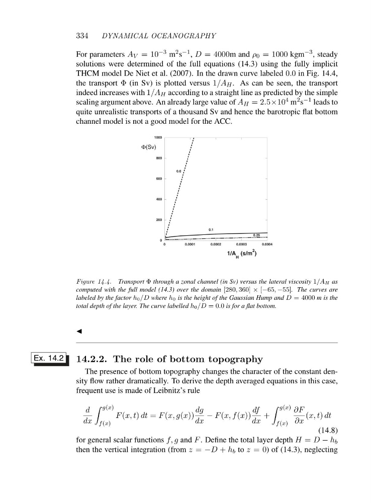
THCM model De Niet et al. (2007). In the drawn curve labeled 0.0 in Fig. 14.4,
the transport Φ (in Sv) is plotted versus 1/A H . As can be seen, the transport
indeed increases with 1/A H according to a straight line as predicted by the simple
scaling argument above. An already large value of A H =2.5×10 4 m 2 s −1 leads to
quite unrealistic transports of a thousand Sv and hence the barotropic flat bottom
channel model is not a good model for the ACC.
0
200
400
600
800
1000
0
0.0001
0.0002
0.0003
0.0004
0.0
0.1
0.25
Φ(Sv)
1/A
H
(s/m
2
)
Figure 14.4. Transport Φ through a zonal channel (in Sv) versus the lateral viscosity 1/AH as
computed with the full model (14.3) over the domain [280, 360] × [−65, −55]. The curves are
labeled by the factor h0/D where h0 is the height of the Gaussian Hump and D = 4000 misthe
total depth of the layer. The curve labelled h0/D =0.0 is for a flat bottom.
◭
14.2.2. The role of bottom topography
Ex. 14.2
The presence of bottom topography changes the character of the constant density flow rather dramatically. To derive the depth averaged equations in this case,
frequent use is made of Leibnitz’s rule
d
dx
g(x)
f (x)
F (x, t) dt = F (x, g(x))
dg
dx
− F (x, f (x))
df
dx
+
g(x)
f (x)
∂F
∂x
(x, t) dt
(14.8)
for general scalar functions f, g and F . Define the total layer depth H = D − h b
then the vertical integration (from z = −D + h b to z =0 ) of (14.3), neglecting
DYNAMICAL OCEANOGRAPHY
For parameters A V =1 0 −3 m 2 s −1 , D = 4000mandρ 0 = 1000 kgm −3 , steady
solutions were determined of the full equations (14.3) using the fully implicit
THCM model De Niet et al. (2007). In the drawn curve labeled 0.0 in Fig. 14.4,
the transport Φ (in Sv) is plotted versus 1/A H . As can be seen, the transport
indeed increases with 1/A H according to a straight line as predicted by the simple
scaling argument above. An already large value of A H =2.5×10 4 m 2 s −1 leads to
quite unrealistic transports of a thousand Sv and hence the barotropic flat bottom
channel model is not a good model for the ACC.
0
200
400
600
800
1000
0
0.0001
0.0002
0.0003
0.0004
0.0
0.1
0.25
Φ(Sv)
1/A
H
(s/m
2
)
Figure 14.4. Transport Φ through a zonal channel (in Sv) versus the lateral viscosity 1/AH as
computed with the full model (14.3) over the domain [280, 360] × [−65, −55]. The curves are
labeled by the factor h0/D where h0 is the height of the Gaussian Hump and D = 4000 misthe
total depth of the layer. The curve labelled h0/D =0.0 is for a flat bottom.
◭
14.2.2. The role of bottom topography
Ex. 14.2
The presence of bottom topography changes the character of the constant density flow rather dramatically. To derive the depth averaged equations in this case,
frequent use is made of Leibnitz’s rule
d
dx
g(x)
f (x)
F (x, t) dt = F (x, g(x))
dg
dx
− F (x, f (x))
df
dx
+
g(x)
f (x)
∂F
∂x
(x, t) dt
(14.8)
for general scalar functions f, g and F . Define the total layer depth H = D − h b
then the vertical integration (from z = −D + h b to z =0 ) of (14.3), neglecting