

304
DYNAMICAL OCEANOGRAPHY
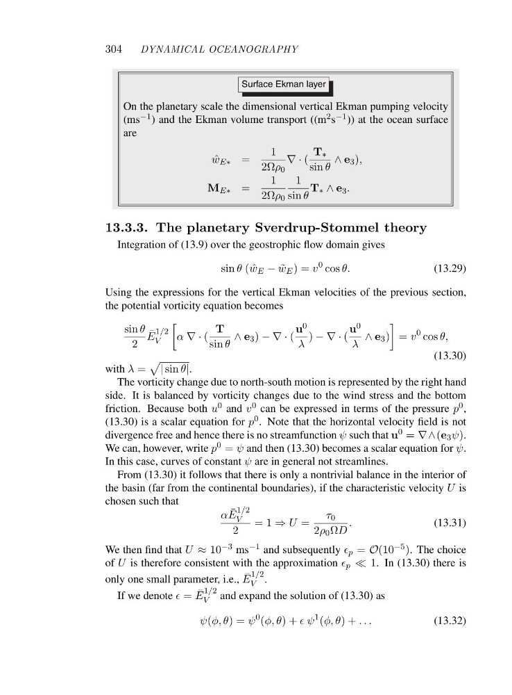
Surface Ekman layer
On the planetary scale the dimensional vertical Ekman pumping velocity
(ms −1 ) and the Ekman volume transport ((m 2 s −1 )) at the ocean surface
are
ˆ
w E∗ =
1
2Ωρ 0
∇·(
T ∗
sin θ
∧ e 3 ),
M E∗ =
1
2Ωρ 0
1
sin θ
T ∗ ∧ e 3 .
13.3.3. The planetary Sverdrup-Stommel theory
Integration of (13.9) over the geostrophic flow domain gives
sin θ (ˆ w E − ˜
w E )=v
0 cos θ.
(13.29)
Using the expressions for the vertical Ekman velocities of the previous section,
the potential vorticity equation becomes
sin θ
2
¯
E
1/2
V
α ∇·(
T
sin θ
∧ e 3 ) −∇·(
u 0
λ
) −∇·(
u 0
λ
∧ e 3 )
= v
0 cos θ,
(13.30)
with λ =
| sin θ|.
The vorticity change due to north-south motion is represented by the right hand
side. It is balanced by vorticity changes due to the wind stress and the bottom
friction. Because both u 0 and v 0 can be expressed in terms of the pressure p 0 ,
(13.30) is a scalar equation for p 0 . Note that the horizontal velocity field is not
divergence free and hence there is no streamfunction ψ such that u 0 = ∇∧(e 3 ψ).
We can, however, write p 0 = ψ and then (13.30) becomes a scalar equation for ψ.
In this case, curves of constant ψ are in general not streamlines.
From (13.30) it follows that there is only a nontrivial balance in the interior of
the basin (far from the continental boundaries), if the characteristic velocity U is
chosen such that
α ¯
E
1/2
V
2
=1⇒ U =
τ 0
2ρ 0 ΩD
.
(13.31)
We then find that U ≈ 10 −3 ms −1 and subsequently ǫ p = O(10 −5 ). The choice
of U is therefore consistent with the approximation ǫ p ≪ 1. In (13.30) there is
only one small parameter, i.e., ¯
E
1/2
V .
If we denote ǫ = ¯
E
1/2
V and expand the solution of (13.30) as
ψ(φ, θ)=ψ
0 (φ, θ)+ǫψ
1 (φ, θ)+...
(13.32)
DYNAMICAL OCEANOGRAPHY
Surface Ekman layer
On the planetary scale the dimensional vertical Ekman pumping velocity
(ms −1 ) and the Ekman volume transport ((m 2 s −1 )) at the ocean surface
are
ˆ
w E∗ =
1
2Ωρ 0
∇·(
T ∗
sin θ
∧ e 3 ),
M E∗ =
1
2Ωρ 0
1
sin θ
T ∗ ∧ e 3 .
13.3.3. The planetary Sverdrup-Stommel theory
Integration of (13.9) over the geostrophic flow domain gives
sin θ (ˆ w E − ˜
w E )=v
0 cos θ.
(13.29)
Using the expressions for the vertical Ekman velocities of the previous section,
the potential vorticity equation becomes
sin θ
2
¯
E
1/2
V
α ∇·(
T
sin θ
∧ e 3 ) −∇·(
u 0
λ
) −∇·(
u 0
λ
∧ e 3 )
= v
0 cos θ,
(13.30)
with λ =
| sin θ|.
The vorticity change due to north-south motion is represented by the right hand
side. It is balanced by vorticity changes due to the wind stress and the bottom
friction. Because both u 0 and v 0 can be expressed in terms of the pressure p 0 ,
(13.30) is a scalar equation for p 0 . Note that the horizontal velocity field is not
divergence free and hence there is no streamfunction ψ such that u 0 = ∇∧(e 3 ψ).
We can, however, write p 0 = ψ and then (13.30) becomes a scalar equation for ψ.
In this case, curves of constant ψ are in general not streamlines.
From (13.30) it follows that there is only a nontrivial balance in the interior of
the basin (far from the continental boundaries), if the characteristic velocity U is
chosen such that
α ¯
E
1/2
V
2
=1⇒ U =
τ 0
2ρ 0 ΩD
.
(13.31)
We then find that U ≈ 10 −3 ms −1 and subsequently ǫ p = O(10 −5 ). The choice
of U is therefore consistent with the approximation ǫ p ≪ 1. In (13.30) there is
only one small parameter, i.e., ¯
E
1/2
V .
If we denote ǫ = ¯
E
1/2
V and expand the solution of (13.30) as
ψ(φ, θ)=ψ
0 (φ, θ)+ǫψ
1 (φ, θ)+...
(13.32)