

Thermocline problem
305
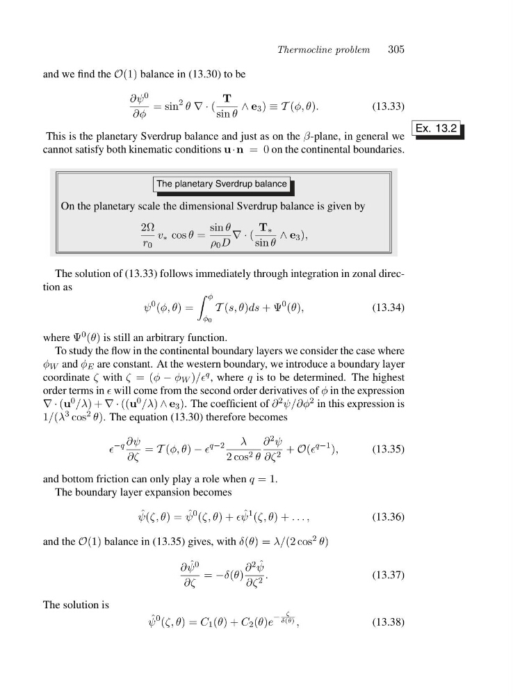
and we find the O(1) balance in (13.30) to be
∂ψ 0
∂φ
=sin
2 θ ∇·(
T
sin θ
∧ e 3 ) ≡T(φ, θ).
(13.33)
This is the planetary Sverdrup balance and just as on the β-plane, in general we
Ex. 13.2
cannot satisfy both kinematic conditions u · n =0on the continental boundaries.
The planetary Sverdrup balance
On the planetary scale the dimensional Sverdrup balance is given by
2Ω
r 0
v ∗ cos θ =
sin θ
ρ 0 D
∇·(
T ∗
sin θ
∧ e 3 ),
The solution of (13.33) follows immediately through integration in zonal direction as
ψ
0 (φ, θ)=
φ
φ0
T (s, θ)ds +Ψ
0 (θ),
(13.34)
where Ψ 0 (θ) is still an arbitrary function.
To study the flow in the continental boundary layers we consider the case where
φ W and φ E are constant. At the western boundary, we introduce a boundary layer
coordinate ζ with ζ =( φ − φ W )/ǫ q , where q is to be determined. The highest
order terms in ǫ will come from the second order derivatives of φ in the expression
∇·(u 0 /λ)+∇·((u 0 /λ) ∧ e 3 ). The coefficient of ∂ 2 ψ/∂φ 2 in this expression is
1/(λ 3 cos 2 θ). The equation (13.30) therefore becomes
ǫ
−q ∂ψ
∂ζ
= T (φ, θ) − ǫ
q−2
λ
2cos 2 θ
∂ 2 ψ
∂ζ 2 + O(ǫ
q−1 ),
(13.35)
and bottom friction can only play a role when q =1.
The boundary layer expansion becomes
ˆ
ψ(ζ,θ)= ˆ
ψ
0 (ζ,θ)+ǫ ˆ
ψ
1 (ζ,θ)+...,
(13.36)
and the O(1) balance in (13.35) gives, with δ(θ)=λ/(2 cos 2 θ)
∂ ˆ
ψ 0
∂ζ
= −δ(θ)
∂ 2 ˆ
ψ
∂ζ 2 .
(13.37)
The solution is
ˆ
ψ
0 (ζ,θ)=C 1 (θ)+C 2 (θ)e
−
ζ
δ(θ) ,
(13.38)
305
and we find the O(1) balance in (13.30) to be
∂ψ 0
∂φ
=sin
2 θ ∇·(
T
sin θ
∧ e 3 ) ≡T(φ, θ).
(13.33)
This is the planetary Sverdrup balance and just as on the β-plane, in general we
Ex. 13.2
cannot satisfy both kinematic conditions u · n =0on the continental boundaries.
The planetary Sverdrup balance
On the planetary scale the dimensional Sverdrup balance is given by
2Ω
r 0
v ∗ cos θ =
sin θ
ρ 0 D
∇·(
T ∗
sin θ
∧ e 3 ),
The solution of (13.33) follows immediately through integration in zonal direction as
ψ
0 (φ, θ)=
φ
φ0
T (s, θ)ds +Ψ
0 (θ),
(13.34)
where Ψ 0 (θ) is still an arbitrary function.
To study the flow in the continental boundary layers we consider the case where
φ W and φ E are constant. At the western boundary, we introduce a boundary layer
coordinate ζ with ζ =( φ − φ W )/ǫ q , where q is to be determined. The highest
order terms in ǫ will come from the second order derivatives of φ in the expression
∇·(u 0 /λ)+∇·((u 0 /λ) ∧ e 3 ). The coefficient of ∂ 2 ψ/∂φ 2 in this expression is
1/(λ 3 cos 2 θ). The equation (13.30) therefore becomes
ǫ
−q ∂ψ
∂ζ
= T (φ, θ) − ǫ
q−2
λ
2cos 2 θ
∂ 2 ψ
∂ζ 2 + O(ǫ
q−1 ),
(13.35)
and bottom friction can only play a role when q =1.
The boundary layer expansion becomes
ˆ
ψ(ζ,θ)= ˆ
ψ
0 (ζ,θ)+ǫ ˆ
ψ
1 (ζ,θ)+...,
(13.36)
and the O(1) balance in (13.35) gives, with δ(θ)=λ/(2 cos 2 θ)
∂ ˆ
ψ 0
∂ζ
= −δ(θ)
∂ 2 ˆ
ψ
∂ζ 2 .
(13.37)
The solution is
ˆ
ψ
0 (ζ,θ)=C 1 (θ)+C 2 (θ)e
−
ζ
δ(θ) ,
(13.38)