

Thermocline problem
303
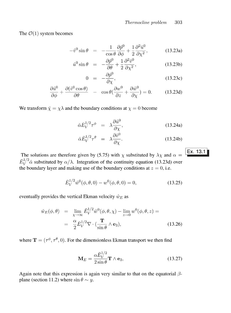
The O(1) system becomes
−ˆ v
0 sin θ = −
1
cos θ
∂ ˆ
p 0
∂φ
+
1
2
∂ 2 ˆ
u 0
∂χ 2 ,
(13.23a)
ˆ
u
0 sin θ = −
∂ ˆ
p 0
∂θ
+
1
2
∂ 2 ˆ
v 0
∂χ 2 ,
(13.23b)
0=−
∂ ˆ
p 0
∂χ
,
(13.23c)
∂ ˆ
u 0
∂φ
+
∂(ˆ v 0 cos θ)
∂θ
− cos θ(
∂w 0
∂z
+
∂ ˆ
w 0
∂χ
)=0.
(13.23d)
We transform ¯
χ = χλ and the boundary conditions at χ =0become
ˆ
α ¯
E
1/2
V τ
φ = λ
∂ ˆ
u 0
∂χ
,
(13.24a)
ˆ
α ¯
E
1/2
V τ
θ = λ
∂ˆ v 0
∂χ
.
(13.24b)
The solutions are therefore given by (5.75) with χ substituted by λχ and α =
Ex. 13.1
¯
E
1/2
V ˆ
α substituted by α/λ. Integration of the continuity equation (13.23d) over
the boundary layer and making use of the boundary conditions at z =0, i.e.
¯
E
1/2
V ˆ
w
0 (φ, θ, 0) − w
0 (φ, θ, 0) = 0,
(13.25)
eventually provides the vertical Ekman velocity ˆ
w E as
ˆ
w E (φ, θ) = lim
χ→∞
¯
E
1/2
V ˆ
w
0 (φ, θ, χ) − lim
z→0
w
0 (φ, θ, z)=
=
α
2
¯
E
1/2
V ∇·(
T
sin θ
∧ e 3 ),
(13.26)
where T =(τ φ ,τ θ , 0). For the dimensionless Ekman transport we then find
M E =
α ¯
E
1/2
V
2sinθ
T ∧ e 3 ,
(13.27)
Again note that this expression is again very similar to that on the equatorial βplane (section 11.2) where sin θ ∼ y.
303
The O(1) system becomes
−ˆ v
0 sin θ = −
1
cos θ
∂ ˆ
p 0
∂φ
+
1
2
∂ 2 ˆ
u 0
∂χ 2 ,
(13.23a)
ˆ
u
0 sin θ = −
∂ ˆ
p 0
∂θ
+
1
2
∂ 2 ˆ
v 0
∂χ 2 ,
(13.23b)
0=−
∂ ˆ
p 0
∂χ
,
(13.23c)
∂ ˆ
u 0
∂φ
+
∂(ˆ v 0 cos θ)
∂θ
− cos θ(
∂w 0
∂z
+
∂ ˆ
w 0
∂χ
)=0.
(13.23d)
We transform ¯
χ = χλ and the boundary conditions at χ =0become
ˆ
α ¯
E
1/2
V τ
φ = λ
∂ ˆ
u 0
∂χ
,
(13.24a)
ˆ
α ¯
E
1/2
V τ
θ = λ
∂ˆ v 0
∂χ
.
(13.24b)
The solutions are therefore given by (5.75) with χ substituted by λχ and α =
Ex. 13.1
¯
E
1/2
V ˆ
α substituted by α/λ. Integration of the continuity equation (13.23d) over
the boundary layer and making use of the boundary conditions at z =0, i.e.
¯
E
1/2
V ˆ
w
0 (φ, θ, 0) − w
0 (φ, θ, 0) = 0,
(13.25)
eventually provides the vertical Ekman velocity ˆ
w E as
ˆ
w E (φ, θ) = lim
χ→∞
¯
E
1/2
V ˆ
w
0 (φ, θ, χ) − lim
z→0
w
0 (φ, θ, z)=
=
α
2
¯
E
1/2
V ∇·(
T
sin θ
∧ e 3 ),
(13.26)
where T =(τ φ ,τ θ , 0). For the dimensionless Ekman transport we then find
M E =
α ¯
E
1/2
V
2sinθ
T ∧ e 3 ,
(13.27)
Again note that this expression is again very similar to that on the equatorial βplane (section 11.2) where sin θ ∼ y.