

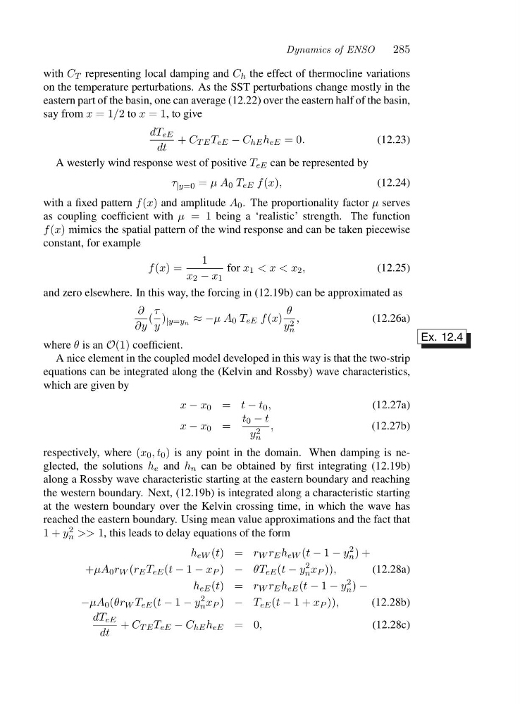
Dynamics of ENSO
285
with C T representing local damping and C h the effect of thermocline variations
on the temperature perturbations. As the SST perturbations change mostly in the
eastern part of the basin, one can average (12.22) over the eastern half of the basin,
say from x =1/2 to x =1,togive
dT eE
dt
+ C TE T eE − C hE h eE =0.
(12.23)
A westerly wind response west of positive T eE can be represented by
τ |y=0 = μA 0 T eE f (x),
(12.24)
with a fixed pattern f (x) and amplitude A 0 . The proportionality factor μ serves
as coupling coefficient with μ =1being a ‘realistic’ strength. The function
f (x) mimics the spatial pattern of the wind response and can be taken piecewise
constant, for example
f (x)=
1
x 2 − x 1
for x 1
and zero elsewhere. In this way, the forcing in (12.19b) can be approximated as
∂
∂y
(
τ
y
) |y=yn ≈−μA 0 T eE f (x)
θ
y 2
n
,
(12.26a)
where θ is an O(1) coefficient.
Ex. 12.4
A nice element in the coupled model developed in this way is that the two-strip
equations can be integrated along the (Kelvin and Rossby) wave characteristics,
which are given by
x − x 0 = t − t 0 ,
(12.27a)
x − x 0 =
t 0 − t
y 2
n
,
(12.27b)
respectively, where (x 0 ,t 0 ) is any point in the domain. When damping is neglected, the solutions h e and h n can be obtained by first integrating (12.19b)
along a Rossby wave characteristic starting at the eastern boundary and reaching
the western boundary. Next, (12.19b) is integrated along a characteristic starting
at the western boundary over the Kelvin crossing time, in which the wave has
reached the eastern boundary. Using mean value approximations and the fact that
1+y 2
n >> 1, this leads to delay equations of the form
h eW (t)=r W r E h eW (t − 1 − y
2
n )+
+μA 0 r W (r E T eE (t − 1 − x P ) − θT eE (t − y
2
n x P )),
(12.28a)
h eE (t)=r W r E h eE (t − 1 − y
2
n ) −
−μA 0 (θr W T eE (t − 1 − y
2
n x P ) − T eE (t − 1+x P )),
(12.28b)
dT eE
dt
+ C TE T eE − C hE h eE =0 ,
(12.28c)
285
with C T representing local damping and C h the effect of thermocline variations
on the temperature perturbations. As the SST perturbations change mostly in the
eastern part of the basin, one can average (12.22) over the eastern half of the basin,
say from x =1/2 to x =1,togive
dT eE
dt
+ C TE T eE − C hE h eE =0.
(12.23)
A westerly wind response west of positive T eE can be represented by
τ |y=0 = μA 0 T eE f (x),
(12.24)
with a fixed pattern f (x) and amplitude A 0 . The proportionality factor μ serves
as coupling coefficient with μ =1being a ‘realistic’ strength. The function
f (x) mimics the spatial pattern of the wind response and can be taken piecewise
constant, for example
f (x)=
1
x 2 − x 1
for x 1
and zero elsewhere. In this way, the forcing in (12.19b) can be approximated as
∂
∂y
(
τ
y
) |y=yn ≈−μA 0 T eE f (x)
θ
y 2
n
,
(12.26a)
where θ is an O(1) coefficient.
Ex. 12.4
A nice element in the coupled model developed in this way is that the two-strip
equations can be integrated along the (Kelvin and Rossby) wave characteristics,
which are given by
x − x 0 = t − t 0 ,
(12.27a)
x − x 0 =
t 0 − t
y 2
n
,
(12.27b)
respectively, where (x 0 ,t 0 ) is any point in the domain. When damping is neglected, the solutions h e and h n can be obtained by first integrating (12.19b)
along a Rossby wave characteristic starting at the eastern boundary and reaching
the western boundary. Next, (12.19b) is integrated along a characteristic starting
at the western boundary over the Kelvin crossing time, in which the wave has
reached the eastern boundary. Using mean value approximations and the fact that
1+y 2
n >> 1, this leads to delay equations of the form
h eW (t)=r W r E h eW (t − 1 − y
2
n )+
+μA 0 r W (r E T eE (t − 1 − x P ) − θT eE (t − y
2
n x P )),
(12.28a)
h eE (t)=r W r E h eE (t − 1 − y
2
n ) −
−μA 0 (θr W T eE (t − 1 − y
2
n x P ) − T eE (t − 1+x P )),
(12.28b)
dT eE
dt
+ C TE T eE − C hE h eE =0 ,
(12.28c)