

284
DYNAMICAL OCEANOGRAPHY
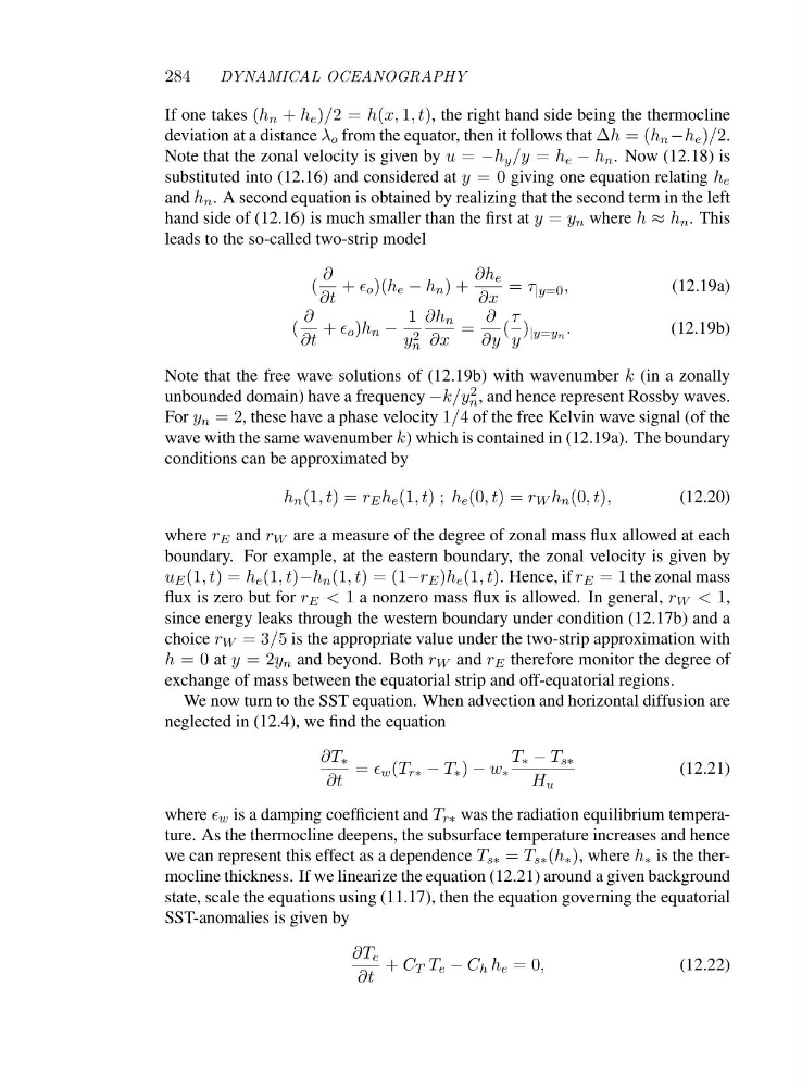
If one takes (h n + h e )/2=h(x, 1,t), the right hand side being the thermocline
deviation at a distance λ o from the equator, then it follows that Δh =(h n −h e )/2.
Note that the zonal velocity is given by u = −h y /y = h e − h n . Now (12.18) is
substituted into (12.16) and considered at y =0giving one equation relating h e
and h n . A second equation is obtained by realizing that the second term in the left
hand side of (12.16) is much smaller than the first at y = y n where h ≈ h n .T h i s
leads to the so-called two-strip model
(
∂
∂t
+ ǫ o )(h e − h n )+
∂h e
∂x
= τ |y=0 ,
(12.19a)
(
∂
∂t
+ ǫ o )h n −
1
y 2
n
∂h n
∂x
=
∂
∂y
(
τ
y
) |y=yn .
(12.19b)
Note that the free wave solutions of (12.19b) with wavenumber k (in a zonally
unbounded domain) have a frequency −k/y 2
n , and hence represent Rossby waves.
For y n =2, these have a phase velocity 1/4 of the free Kelvin wave signal (of the
wave with the same wavenumber k) which is contained in (12.19a). The boundary
conditions can be approximated by
h n (1,t)=r E h e (1,t); h e (0,t)=r W h n (0,t),
(12.20)
where r E and r W are a measure of the degree of zonal mass flux allowed at each
boundary. For example, at the eastern boundary, the zonal velocity is given by
u E (1,t)=h e (1,t)−h n (1,t)=(1−r E )h e (1,t). Hence, if r E =1the zonal mass
flux is zero but for r E < 1 a nonzero mass flux is allowed. In general, r W < 1,
since energy leaks through the western boundary under condition (12.17b) and a
choice r W =3/5 is the appropriate value under the two-strip approximation with
h =0at y =2 y n and beyond. Both r W and r E therefore monitor the degree of
exchange of mass between the equatorial strip and off-equatorial regions.
We now turn to the SST equation. When advection and horizontal diffusion are
neglected in (12.4), we find the equation
∂T ∗
∂t
= ǫ w (T r∗ − T ∗ ) − w ∗
T ∗ − T s∗
H u
(12.21)
where ǫ w is a damping coefficient and T r∗ was the radiation equilibrium temperature. As the thermocline deepens, the subsurface temperature increases and hence
we can represent this effect as a dependence T s∗ = T s∗ (h ∗ ), where h ∗ is the thermocline thickness. If we linearize the equation (12.21) around a given background
state, scale the equations using (11.17), then the equation governing the equatorial
SST-anomalies is given by
∂T e
∂t
+ C T T e − C h h e =0,
(12.22)
DYNAMICAL OCEANOGRAPHY
If one takes (h n + h e )/2=h(x, 1,t), the right hand side being the thermocline
deviation at a distance λ o from the equator, then it follows that Δh =(h n −h e )/2.
Note that the zonal velocity is given by u = −h y /y = h e − h n . Now (12.18) is
substituted into (12.16) and considered at y =0giving one equation relating h e
and h n . A second equation is obtained by realizing that the second term in the left
hand side of (12.16) is much smaller than the first at y = y n where h ≈ h n .T h i s
leads to the so-called two-strip model
(
∂
∂t
+ ǫ o )(h e − h n )+
∂h e
∂x
= τ |y=0 ,
(12.19a)
(
∂
∂t
+ ǫ o )h n −
1
y 2
n
∂h n
∂x
=
∂
∂y
(
τ
y
) |y=yn .
(12.19b)
Note that the free wave solutions of (12.19b) with wavenumber k (in a zonally
unbounded domain) have a frequency −k/y 2
n , and hence represent Rossby waves.
For y n =2, these have a phase velocity 1/4 of the free Kelvin wave signal (of the
wave with the same wavenumber k) which is contained in (12.19a). The boundary
conditions can be approximated by
h n (1,t)=r E h e (1,t); h e (0,t)=r W h n (0,t),
(12.20)
where r E and r W are a measure of the degree of zonal mass flux allowed at each
boundary. For example, at the eastern boundary, the zonal velocity is given by
u E (1,t)=h e (1,t)−h n (1,t)=(1−r E )h e (1,t). Hence, if r E =1the zonal mass
flux is zero but for r E < 1 a nonzero mass flux is allowed. In general, r W < 1,
since energy leaks through the western boundary under condition (12.17b) and a
choice r W =3/5 is the appropriate value under the two-strip approximation with
h =0at y =2 y n and beyond. Both r W and r E therefore monitor the degree of
exchange of mass between the equatorial strip and off-equatorial regions.
We now turn to the SST equation. When advection and horizontal diffusion are
neglected in (12.4), we find the equation
∂T ∗
∂t
= ǫ w (T r∗ − T ∗ ) − w ∗
T ∗ − T s∗
H u
(12.21)
where ǫ w is a damping coefficient and T r∗ was the radiation equilibrium temperature. As the thermocline deepens, the subsurface temperature increases and hence
we can represent this effect as a dependence T s∗ = T s∗ (h ∗ ), where h ∗ is the thermocline thickness. If we linearize the equation (12.21) around a given background
state, scale the equations using (11.17), then the equation governing the equatorial
SST-anomalies is given by
∂T e
∂t
+ C T T e − C h h e =0,
(12.22)