

Dynamics of ENSO
283
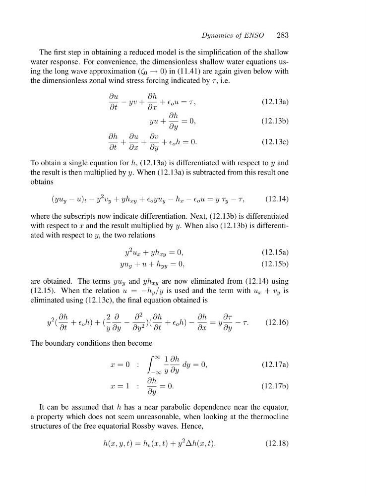
The first step in obtaining a reduced model is the simplification of the shallow
water response. For convenience, the dimensionless shallow water equations using the long wave approximation (ζ 0 → 0) in (11.41) are again given below with
the dimensionless zonal wind stress forcing indicated by τ , i.e.
∂u
∂t
− yv +
∂h
∂x
+ ǫ o u = τ,
(12.13a)
yu +
∂h
∂y
=0,
(12.13b)
∂h
∂t
+
∂u
∂x
+
∂v
∂y
+ ǫ o h =0.
(12.13c)
To obtain a single equation for h, (12.13a) is differentiated with respect to y and
the result is then multiplied by y. When (12.13a) is subtracted from this result one
obtains
(yu y − u) t − y
2 v y + yh xy + ǫ o yu y − h x − ǫ o u = yτ y − τ,
(12.14)
where the subscripts now indicate differentiation. Next, (12.13b) is differentiated
with respect to x and the result multiplied by y. When also (12.13b) is differentiated with respect to y, the two relations
y
2 u x + yh xy =0,
(12.15a)
yu y + u + h yy =0,
(12.15b)
are obtained. The terms yu y and yh xy are now eliminated from (12.14) using
(12.15). When the relation u = −h y /y is used and the term with u x + v y is
eliminated using (12.13c), the final equation obtained is
y
2 (
∂h
∂t
+ ǫ o h)+(
2
y
∂
∂y
−
∂ 2
∂y 2 )(
∂h
∂t
+ ǫ o h) −
∂h
∂x
= y
∂τ
∂y
− τ.
(12.16)
The boundary conditions then become
x =0 :
∞
−∞
1
y
∂h
∂y
dy =0,
(12.17a)
x =1 :
∂h
∂y
=0.
(12.17b)
It can be assumed that h has a near parabolic dependence near the equator,
a property which does not seem unreasonable, when looking at the thermocline
structures of the free equatorial Rossby waves. Hence,
h(x, y, t)=h e (x, t)+y
2 Δh(x, t).
(12.18)
283
The first step in obtaining a reduced model is the simplification of the shallow
water response. For convenience, the dimensionless shallow water equations using the long wave approximation (ζ 0 → 0) in (11.41) are again given below with
the dimensionless zonal wind stress forcing indicated by τ , i.e.
∂u
∂t
− yv +
∂h
∂x
+ ǫ o u = τ,
(12.13a)
yu +
∂h
∂y
=0,
(12.13b)
∂h
∂t
+
∂u
∂x
+
∂v
∂y
+ ǫ o h =0.
(12.13c)
To obtain a single equation for h, (12.13a) is differentiated with respect to y and
the result is then multiplied by y. When (12.13a) is subtracted from this result one
obtains
(yu y − u) t − y
2 v y + yh xy + ǫ o yu y − h x − ǫ o u = yτ y − τ,
(12.14)
where the subscripts now indicate differentiation. Next, (12.13b) is differentiated
with respect to x and the result multiplied by y. When also (12.13b) is differentiated with respect to y, the two relations
y
2 u x + yh xy =0,
(12.15a)
yu y + u + h yy =0,
(12.15b)
are obtained. The terms yu y and yh xy are now eliminated from (12.14) using
(12.15). When the relation u = −h y /y is used and the term with u x + v y is
eliminated using (12.13c), the final equation obtained is
y
2 (
∂h
∂t
+ ǫ o h)+(
2
y
∂
∂y
−
∂ 2
∂y 2 )(
∂h
∂t
+ ǫ o h) −
∂h
∂x
= y
∂τ
∂y
− τ.
(12.16)
The boundary conditions then become
x =0 :
∞
−∞
1
y
∂h
∂y
dy =0,
(12.17a)
x =1 :
∂h
∂y
=0.
(12.17b)
It can be assumed that h has a near parabolic dependence near the equator,
a property which does not seem unreasonable, when looking at the thermocline
structures of the free equatorial Rossby waves. Hence,
h(x, y, t)=h e (x, t)+y
2 Δh(x, t).
(12.18)