

Equatorial ocean circulation
267
where ˜
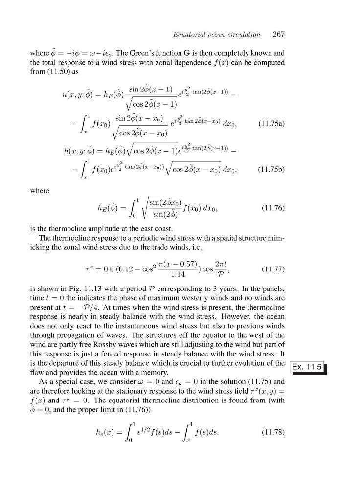
φ = −iφ = ω −iǫ o . The Green’s function G is then completely known and
the total response to a wind stress with zonal dependence f (x) can be computed
from (11.50) as
u(x, y; ˜
φ)=h E ( ˜
φ)
sin 2 ˜
φ(x − 1)
cos 2 ˜
φ(x − 1)
e
i
y 2
2
tan(2 ˜
φ(x−1)) −
−
1
x
f (x 0 )
sin 2 ˜
φ(x − x 0 )
cos 2 ˜
φ(x − x 0 )
e
i
y 2
2
tan 2 ˜
φ(x−x0) dx 0 ,
(11.75a)
h(x, y; ˜
φ)=h E ( ˜
φ)
cos 2 ˜
φ(x − 1)e
i
y 2
2
tan(2 ˜
φ(x−1)) −
−
1
x
f (x 0 )e
i
y 2
2
tan(2 ˜
φ(x−x0))
cos 2 ˜
φ(x − x 0 ) dx 0 ,
(11.75b)
where
h E ( ˜
φ)=
1
0
sin(2 ˜
φx 0 )
sin(2 ˜
φ)
f (x 0 ) dx 0 ,
(11.76)
is the thermocline amplitude at the east coast.
The thermocline response to a periodic wind stress with a spatial structure mimicking the zonal wind stress due to the trade winds, i.e.,
τ
x =0.6(0.12 − cos
2 π(x − 0.57)
1.14
)cos
2πt
P
,
(11.77)
is shown in Fig. 11.13 with a period P corresponding to 3 years. In the panels,
time t =0the indicates the phase of maximum westerly winds and no winds are
present at t = −P/4. At times when the wind stress is present, the thermocline
response is nearly in steady balance with the wind stress. However, the ocean
does not only react to the instantaneous wind stress but also to previous winds
through propagation of waves. The structures off the equator to the west of the
wind are partly free Rossby waves which are still adjusting to the wind but part of
this response is just a forced response in steady balance with the wind stress. It
is the departure of this steady balance which is crucial to further evolution of the
flow and provides the ocean with a memory.
Ex. 11.5
As a special case, we consider ω =0and ǫ o =0in the solution (11.75) and
are therefore looking at the stationary response to the wind stress field τ x (x, y)=
f (x) and τ y =0 . The equatorial thermocline distribution is found from (with
˜
φ =0, and the proper limit in (11.76))
h e (x)=
1
0
s
1/2 f (s)ds −
1
x
f (s)ds.
(11.78)
267
where ˜
φ = −iφ = ω −iǫ o . The Green’s function G is then completely known and
the total response to a wind stress with zonal dependence f (x) can be computed
from (11.50) as
u(x, y; ˜
φ)=h E ( ˜
φ)
sin 2 ˜
φ(x − 1)
cos 2 ˜
φ(x − 1)
e
i
y 2
2
tan(2 ˜
φ(x−1)) −
−
1
x
f (x 0 )
sin 2 ˜
φ(x − x 0 )
cos 2 ˜
φ(x − x 0 )
e
i
y 2
2
tan 2 ˜
φ(x−x0) dx 0 ,
(11.75a)
h(x, y; ˜
φ)=h E ( ˜
φ)
cos 2 ˜
φ(x − 1)e
i
y 2
2
tan(2 ˜
φ(x−1)) −
−
1
x
f (x 0 )e
i
y 2
2
tan(2 ˜
φ(x−x0))
cos 2 ˜
φ(x − x 0 ) dx 0 ,
(11.75b)
where
h E ( ˜
φ)=
1
0
sin(2 ˜
φx 0 )
sin(2 ˜
φ)
f (x 0 ) dx 0 ,
(11.76)
is the thermocline amplitude at the east coast.
The thermocline response to a periodic wind stress with a spatial structure mimicking the zonal wind stress due to the trade winds, i.e.,
τ
x =0.6(0.12 − cos
2 π(x − 0.57)
1.14
)cos
2πt
P
,
(11.77)
is shown in Fig. 11.13 with a period P corresponding to 3 years. In the panels,
time t =0the indicates the phase of maximum westerly winds and no winds are
present at t = −P/4. At times when the wind stress is present, the thermocline
response is nearly in steady balance with the wind stress. However, the ocean
does not only react to the instantaneous wind stress but also to previous winds
through propagation of waves. The structures off the equator to the west of the
wind are partly free Rossby waves which are still adjusting to the wind but part of
this response is just a forced response in steady balance with the wind stress. It
is the departure of this steady balance which is crucial to further evolution of the
flow and provides the ocean with a memory.
Ex. 11.5
As a special case, we consider ω =0and ǫ o =0in the solution (11.75) and
are therefore looking at the stationary response to the wind stress field τ x (x, y)=
f (x) and τ y =0 . The equatorial thermocline distribution is found from (with
˜
φ =0, and the proper limit in (11.76))
h e (x)=
1
0
s
1/2 f (s)ds −
1
x
f (s)ds.
(11.78)