

266
DYNAMICAL OCEANOGRAPHY
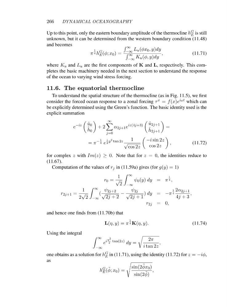
Up to this point, only the eastern boundary amplitude of the thermocline h G
E is still
unknown, but it can be determined from the western boundary condition (11.48)
and becomes
π
1
4 h
G
E (φ; x 0 )=
∞
−∞ L u (φx 0 ,y)dy
∞
−∞ K u (φ, y)dy
,
(11.71)
where K u and L u are the first components of K and L, respectively. This completes the basic machinery needed in the next section to understand the response
of the ocean to varying wind stress forcing.
11.6. The equatorial thermocline
To understand the spatial structure of the thermocline (as in Fig. 11.5), we first
consider the forced ocean response to a zonal forcing τ x = f (x)e iωt which can
be explicitly determined using the Green’s function. The basic identity used is the
explicit summation
e
−iz
ˆ
u 0
ˆ
h 0
+2
∞
j=0
α 2j+1 e
iz(4j+3)
ˆ
u 2j+1
ˆ
h 2j+1
=
= π
−
1
4 e
i
2
y 2 tan 2z
1
√
cos 2z
−i sin 2z
cos 2z
,
(11.72)
for complex z with Im(z) ≥ 0. Note that for z =0 , the identities reduce to
(11.67).
Computation of the values of r j in (11.59a) gives (for g(y)=1)
r 0 =
1
√
2
∞
−∞
ψ 0 (y) dy = π
1
4 ,
r 2j+1 =
1
2
√
2
∞
−∞
(
ψ 2j+2
√ 2j +2
−
ψ 2j
√ 2j +1
) dy = −π
1
4
2α 2j+1
4j +3
,
r 2j =0 ,
and hence one finds from (11.70b) that
L(η, y)=π
1
4 K(η, y).
(11.74)
Using the integral
∞
−∞
e
i
y 2
2
tan(2z) dy =
2π
i tan 2z
,
one obtains as a solution for h G
E in (11.71), using the identity (11.72) for z = −iφ,
as
h
G
E ( ˜
φ; x 0 )=
sin(2 ˜
φx 0 )
sin(2 ˜
φ)
,
DYNAMICAL OCEANOGRAPHY
Up to this point, only the eastern boundary amplitude of the thermocline h G
E is still
unknown, but it can be determined from the western boundary condition (11.48)
and becomes
π
1
4 h
G
E (φ; x 0 )=
∞
−∞ L u (φx 0 ,y)dy
∞
−∞ K u (φ, y)dy
,
(11.71)
where K u and L u are the first components of K and L, respectively. This completes the basic machinery needed in the next section to understand the response
of the ocean to varying wind stress forcing.
11.6. The equatorial thermocline
To understand the spatial structure of the thermocline (as in Fig. 11.5), we first
consider the forced ocean response to a zonal forcing τ x = f (x)e iωt which can
be explicitly determined using the Green’s function. The basic identity used is the
explicit summation
e
−iz
ˆ
u 0
ˆ
h 0
+2
∞
j=0
α 2j+1 e
iz(4j+3)
ˆ
u 2j+1
ˆ
h 2j+1
=
= π
−
1
4 e
i
2
y 2 tan 2z
1
√
cos 2z
−i sin 2z
cos 2z
,
(11.72)
for complex z with Im(z) ≥ 0. Note that for z =0 , the identities reduce to
(11.67).
Computation of the values of r j in (11.59a) gives (for g(y)=1)
r 0 =
1
√
2
∞
−∞
ψ 0 (y) dy = π
1
4 ,
r 2j+1 =
1
2
√
2
∞
−∞
(
ψ 2j+2
√ 2j +2
−
ψ 2j
√ 2j +1
) dy = −π
1
4
2α 2j+1
4j +3
,
r 2j =0 ,
and hence one finds from (11.70b) that
L(η, y)=π
1
4 K(η, y).
(11.74)
Using the integral
∞
−∞
e
i
y 2
2
tan(2z) dy =
2π
i tan 2z
,
one obtains as a solution for h G
E in (11.71), using the identity (11.72) for z = −iφ,
as
h
G
E ( ˜
φ; x 0 )=
sin(2 ˜
φx 0 )
sin(2 ˜
φ)
,