

Equatorial ocean circulation
265
while for x
−φ(x−x0) +
(11.64)
+
∞
j=1
((2j +1)r j + b j )e
φ(2j+1)(x−x0) Φ j (y).
(11.65)
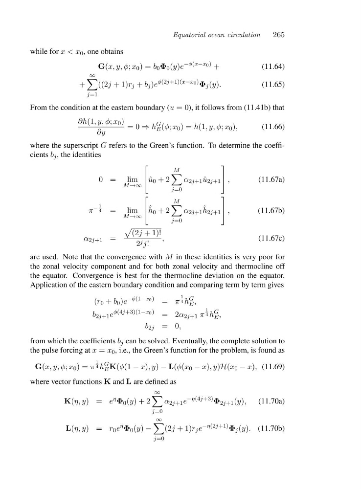
From the condition at the eastern boundary (u =0), it follows from (11.41b) that
∂h(1,y,φ; x 0 )
∂y
=0⇒ h
G
E (φ; x 0 )=h(1,y,φ; x 0 ),
(11.66)
where the superscript G refers to the Green’s function. To determine the coefficients b j , the identities
0 = lim
M →∞
⎡
⎣ ˆ
u 0 +2
M
j=0
α 2j+1 ˆ
u 2j+1
⎤
⎦ ,
(11.67a)
π
−
1
4
= lim
M →∞
⎡
⎣ˆ h 0 +2
M
j=0
α 2j+1 ˆ
h 2j+1
⎤
⎦ ,
(11.67b)
α 2j+1 =
(2j +1)!
2 j j!
,
(11.67c)
are used. Note that the convergence with M in these identities is very poor for
the zonal velocity component and for both zonal velocity and thermocline off
the equator. Convergence is best for the thermocline deviation on the equator.
Application of the eastern boundary condition and comparing term by term gives
(r 0 + b 0 )e
−φ(1−x0) = π
1
4 h
G
E ,
b 2j+1 e
φ(4j+3)(1−x0) =2 α 2j+1 π
1
4 h
G
E ,
b 2j =0 ,
from which the coefficients b j can be solved. Eventually, the complete solution to
the pulse forcing at x = x 0 , i.e., the Green’s function for the problem, is found as
G(x, y, φ; x 0 )=π
1
4 h
G
E K(φ(1 − x),y) − L(φ(x 0 − x),y)H(x 0 − x), (11.69)
where vector functions K and L are defined as
K(η, y)=e
η Φ 0 (y)+2
∞
j=0
α 2j+1 e
−η(4j+3) Φ 2j+1 (y),
(11.70a)
L(η, y)=r 0 e
η Φ 0 (y) −
∞
j=0
(2j +1)r j e
−η(2j+1) Φ j (y). (11.70b)
265
while for x
−φ(x−x0) +
(11.64)
+
∞
j=1
((2j +1)r j + b j )e
φ(2j+1)(x−x0) Φ j (y).
(11.65)
From the condition at the eastern boundary (u =0), it follows from (11.41b) that
∂h(1,y,φ; x 0 )
∂y
=0⇒ h
G
E (φ; x 0 )=h(1,y,φ; x 0 ),
(11.66)
where the superscript G refers to the Green’s function. To determine the coefficients b j , the identities
0 = lim
M →∞
⎡
⎣ ˆ
u 0 +2
M
j=0
α 2j+1 ˆ
u 2j+1
⎤
⎦ ,
(11.67a)
π
−
1
4
= lim
M →∞
⎡
⎣ˆ h 0 +2
M
j=0
α 2j+1 ˆ
h 2j+1
⎤
⎦ ,
(11.67b)
α 2j+1 =
(2j +1)!
2 j j!
,
(11.67c)
are used. Note that the convergence with M in these identities is very poor for
the zonal velocity component and for both zonal velocity and thermocline off
the equator. Convergence is best for the thermocline deviation on the equator.
Application of the eastern boundary condition and comparing term by term gives
(r 0 + b 0 )e
−φ(1−x0) = π
1
4 h
G
E ,
b 2j+1 e
φ(4j+3)(1−x0) =2 α 2j+1 π
1
4 h
G
E ,
b 2j =0 ,
from which the coefficients b j can be solved. Eventually, the complete solution to
the pulse forcing at x = x 0 , i.e., the Green’s function for the problem, is found as
G(x, y, φ; x 0 )=π
1
4 h
G
E K(φ(1 − x),y) − L(φ(x 0 − x),y)H(x 0 − x), (11.69)
where vector functions K and L are defined as
K(η, y)=e
η Φ 0 (y)+2
∞
j=0
α 2j+1 e
−η(4j+3) Φ 2j+1 (y),
(11.70a)
L(η, y)=r 0 e
η Φ 0 (y) −
∞
j=0
(2j +1)r j e
−η(2j+1) Φ j (y). (11.70b)