264
DYNAMICAL OCEANOGRAPHY
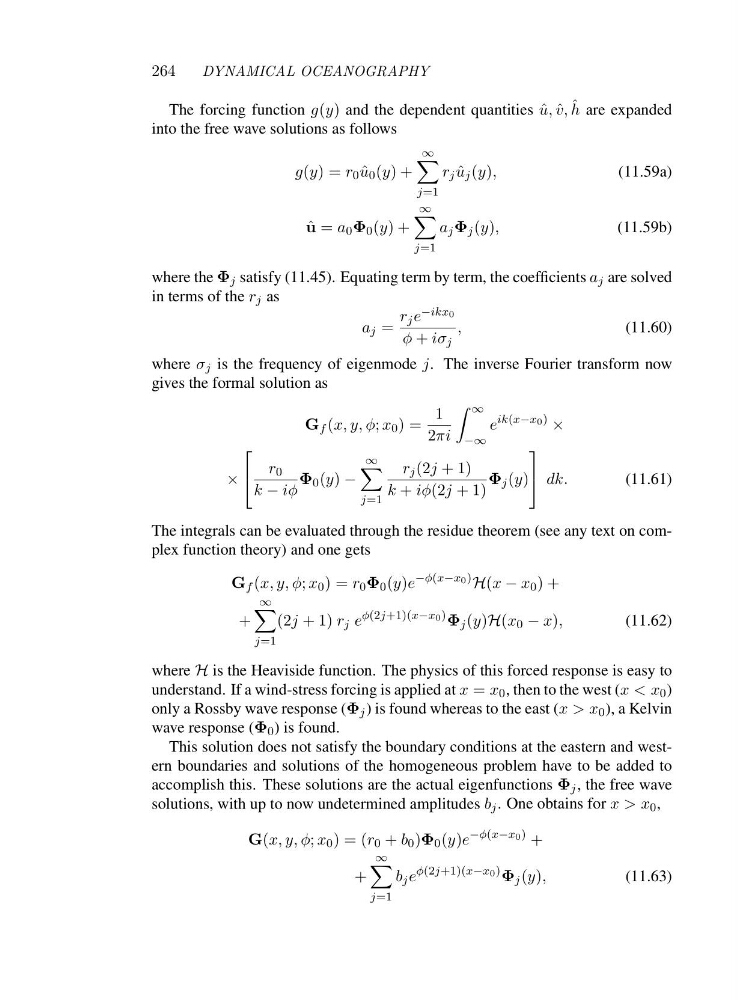
The forcing function g(y) and the dependent quantities ˆ
u, ˆ
v, ˆ
h are expanded
into the free wave solutions as follows
g(y)=r 0 ˆ
u 0 (y)+
∞
j=1
r j ˆ
u j (y),
(11.59a)
ˆ
u = a 0 Φ 0 (y)+
∞
j=1
a j Φ j (y),
(11.59b)
where the Φ j satisfy (11.45). Equating term by term, the coefficients a j are solved
in terms of the r j as
a j =
r j e −ikx0
φ + iσ j
,
(11.60)
where σ j is the frequency of eigenmode j. The inverse Fourier transform now
gives the formal solution as
G f (x, y, φ; x 0 )=
1
2πi
∞
−∞
e
ik(x−x0) ×
×
⎡
⎣ r 0
k − iφ
Φ 0 (y) −
∞
j=1
r j (2j +1)
k + iφ(2j +1)
Φ j (y)
⎤
⎦ dk.
(11.61)
The integrals can be evaluated through the residue theorem (see any text on complex function theory) and one gets
G f (x, y, φ; x 0 )=r 0 Φ 0 (y)e
−φ(x−x0) H(x − x 0 )+
+
∞
j=1
(2j +1)r j e
φ(2j+1)(x−x0) Φ j (y)H(x 0 − x),
(11.62)
where H is the Heaviside function. The physics of this forced response is easy to
understand. If a wind-stress forcing is applied at x = x 0 , then to the west (x only a Rossby wave response (Φ j ) is found whereas to the east (x>x 0 ), a Kelvin
wave response (Φ 0 ) is found.
This solution does not satisfy the boundary conditions at the eastern and western boundaries and solutions of the homogeneous problem have to be added to
accomplish this. These solutions are the actual eigenfunctions Φ j , the free wave
solutions, with up to now undetermined amplitudes b j . One obtains for x>x 0 ,
G(x, y, φ; x 0 )=(r 0 + b 0 )Φ 0 (y)e
−φ(x−x0) +
+
∞
j=1
b j e
φ(2j+1)(x−x0) Φ j (y),
(11.63)