

Equatorial ocean circulation
263
as
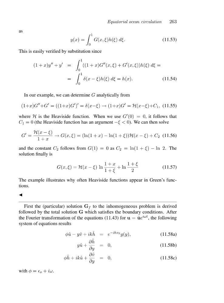
y(x)=
1
0
G(x, ξ)h(ξ) dξ.
(11.53)
This is easily verified by substitution since
(1 + x)y
′′ + y
′ =
1
0
((1 + x)G
′′ (x, ξ)+G
′ (x, ξ))h(ξ) dξ =
=
1
0
δ(x − ξ)h(ξ) dξ = h(x).
(11.54)
In our example, we can determine G analytically from
(1+x)G
′′ +G
′ = ((1+x)G
′ )
′ = δ(x−ξ) → (1+x)G
′ = H(x−ξ)+C 1 , (11.55)
where H is the Heaviside function. When we use G ′ (0) = 0, it follows that
C 1 =0(the Heaviside function has an argument −ξ<0). We can then solve
G
′ =
H(x − ξ)
1+x
→ G(x, ξ)=(ln(1+x) − ln(1 + ξ))H(x − ξ)+C 2 (11.56)
and the constant C 2 follows from G(1) = 0 as C 2 = ln(1 + ξ) − ln 2.T h e
solution finally is
G(x, ξ)=H(x − ξ)l n
1+x
1+ξ
+ln
1+ξ
2
(11.57)
The example illustrates why often Heaviside functions appear in Green’s functions.
◭
First the (particular) solution G f to the inhomogeneous problem is derived
followed by the total solution G which satisfies the boundary conditions. After
the Fourier transformation of the equations (11.43) for u = ˜
ue iωt , the following
system of equations results
φˆ u − yˆ v + ik ˆ
h = e
−ikx0 g(y),
(11.58a)
yˆ u +
∂ ˆ
h
∂y
=0 ,
(11.58b)
φ ˆ
h + ikˆ u +
∂ˆ v
∂y
=0 ,
(11.58c)
with φ = ǫ o + iω.
263
as
y(x)=
1
0
G(x, ξ)h(ξ) dξ.
(11.53)
This is easily verified by substitution since
(1 + x)y
′′ + y
′ =
1
0
((1 + x)G
′′ (x, ξ)+G
′ (x, ξ))h(ξ) dξ =
=
1
0
δ(x − ξ)h(ξ) dξ = h(x).
(11.54)
In our example, we can determine G analytically from
(1+x)G
′′ +G
′ = ((1+x)G
′ )
′ = δ(x−ξ) → (1+x)G
′ = H(x−ξ)+C 1 , (11.55)
where H is the Heaviside function. When we use G ′ (0) = 0, it follows that
C 1 =0(the Heaviside function has an argument −ξ<0). We can then solve
G
′ =
H(x − ξ)
1+x
→ G(x, ξ)=(ln(1+x) − ln(1 + ξ))H(x − ξ)+C 2 (11.56)
and the constant C 2 follows from G(1) = 0 as C 2 = ln(1 + ξ) − ln 2.T h e
solution finally is
G(x, ξ)=H(x − ξ)l n
1+x
1+ξ
+ln
1+ξ
2
(11.57)
The example illustrates why often Heaviside functions appear in Green’s functions.
◭
First the (particular) solution G f to the inhomogeneous problem is derived
followed by the total solution G which satisfies the boundary conditions. After
the Fourier transformation of the equations (11.43) for u = ˜
ue iωt , the following
system of equations results
φˆ u − yˆ v + ik ˆ
h = e
−ikx0 g(y),
(11.58a)
yˆ u +
∂ ˆ
h
∂y
=0 ,
(11.58b)
φ ˆ
h + ikˆ u +
∂ˆ v
∂y
=0 ,
(11.58c)
with φ = ǫ o + iω.