

262
DYNAMICAL OCEANOGRAPHY
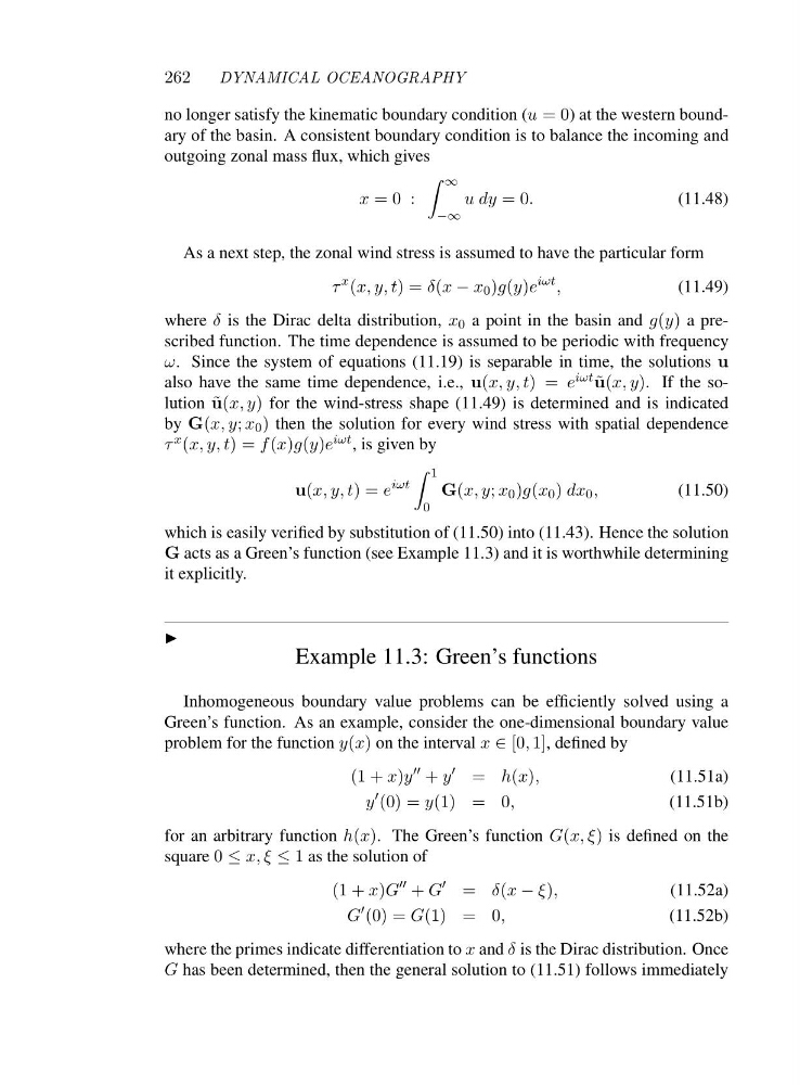
no longer satisfy the kinematic boundary condition (u =0) at the western boundary of the basin. A consistent boundary condition is to balance the incoming and
outgoing zonal mass flux, which gives
x =0 :
∞
−∞
udy=0.
(11.48)
As a next step, the zonal wind stress is assumed to have the particular form
τ
x (x, y, t)=δ(x − x 0 )g(y)e
iωt ,
(11.49)
where δ is the Dirac delta distribution, x 0 a point in the basin and g(y) ap r e -
scribed function. The time dependence is assumed to be periodic with frequency
ω. Since the system of equations (11.19) is separable in time, the solutions u
also have the same time dependence, i.e., u(x, y, t)=e iωt ˜
u(x, y).I f t h e s o -
lution ˜
u(x, y) for the wind-stress shape (11.49) is determined and is indicated
by G(x, y; x 0 ) then the solution for every wind stress with spatial dependence
τ x (x, y, t)=f (x)g(y)e iωt ,isgivenby
u(x, y, t)=e
iωt
1
0
G(x, y; x 0 )g(x 0 ) dx 0 ,
(11.50)
which is easily verified by substitution of (11.50) into (11.43). Hence the solution
G acts as a Green’s function (see Example 11.3) and it is worthwhile determining
it explicitly.
◮
Example 11.3: Green’s functions
Inhomogeneous boundary value problems can be efficiently solved using a
Green’s function. As an example, consider the one-dimensional boundary value
problem for the function y(x) on the interval x ∈ [0, 1],definedby
(1 + x)y
′′ + y
′ = h(x),
(11.51a)
y
′ (0) = y(1) = 0,
(11.51b)
for an arbitrary function h(x). The Green’s function G(x, ξ) is defined on the
square 0 ≤ x, ξ ≤ 1 as the solution of
(1 + x)G
′′ + G
′ = δ(x − ξ),
(11.52a)
G
′ (0) = G(1) = 0,
(11.52b)
where the primes indicate differentiation to x and δ is the Dirac distribution. Once
G has been determined, then the general solution to (11.51) follows immediately
DYNAMICAL OCEANOGRAPHY
no longer satisfy the kinematic boundary condition (u =0) at the western boundary of the basin. A consistent boundary condition is to balance the incoming and
outgoing zonal mass flux, which gives
x =0 :
∞
−∞
udy=0.
(11.48)
As a next step, the zonal wind stress is assumed to have the particular form
τ
x (x, y, t)=δ(x − x 0 )g(y)e
iωt ,
(11.49)
where δ is the Dirac delta distribution, x 0 a point in the basin and g(y) ap r e -
scribed function. The time dependence is assumed to be periodic with frequency
ω. Since the system of equations (11.19) is separable in time, the solutions u
also have the same time dependence, i.e., u(x, y, t)=e iωt ˜
u(x, y).I f t h e s o -
lution ˜
u(x, y) for the wind-stress shape (11.49) is determined and is indicated
by G(x, y; x 0 ) then the solution for every wind stress with spatial dependence
τ x (x, y, t)=f (x)g(y)e iωt ,isgivenby
u(x, y, t)=e
iωt
1
0
G(x, y; x 0 )g(x 0 ) dx 0 ,
(11.50)
which is easily verified by substitution of (11.50) into (11.43). Hence the solution
G acts as a Green’s function (see Example 11.3) and it is worthwhile determining
it explicitly.
◮
Example 11.3: Green’s functions
Inhomogeneous boundary value problems can be efficiently solved using a
Green’s function. As an example, consider the one-dimensional boundary value
problem for the function y(x) on the interval x ∈ [0, 1],definedby
(1 + x)y
′′ + y
′ = h(x),
(11.51a)
y
′ (0) = y(1) = 0,
(11.51b)
for an arbitrary function h(x). The Green’s function G(x, ξ) is defined on the
square 0 ≤ x, ξ ≤ 1 as the solution of
(1 + x)G
′′ + G
′ = δ(x − ξ),
(11.52a)
G
′ (0) = G(1) = 0,
(11.52b)
where the primes indicate differentiation to x and δ is the Dirac distribution. Once
G has been determined, then the general solution to (11.51) follows immediately