

Equatorial ocean circulation
261
L =
⎛
⎝
ǫ o −y
∂
∂x
yζ o ǫ o
∂
∂y
∂
∂x
∂
∂y
ǫ o
⎞
⎠
; M =
⎛
⎝
100
0 ζ 2
o
0
001
⎞
⎠ .
(11.43b)
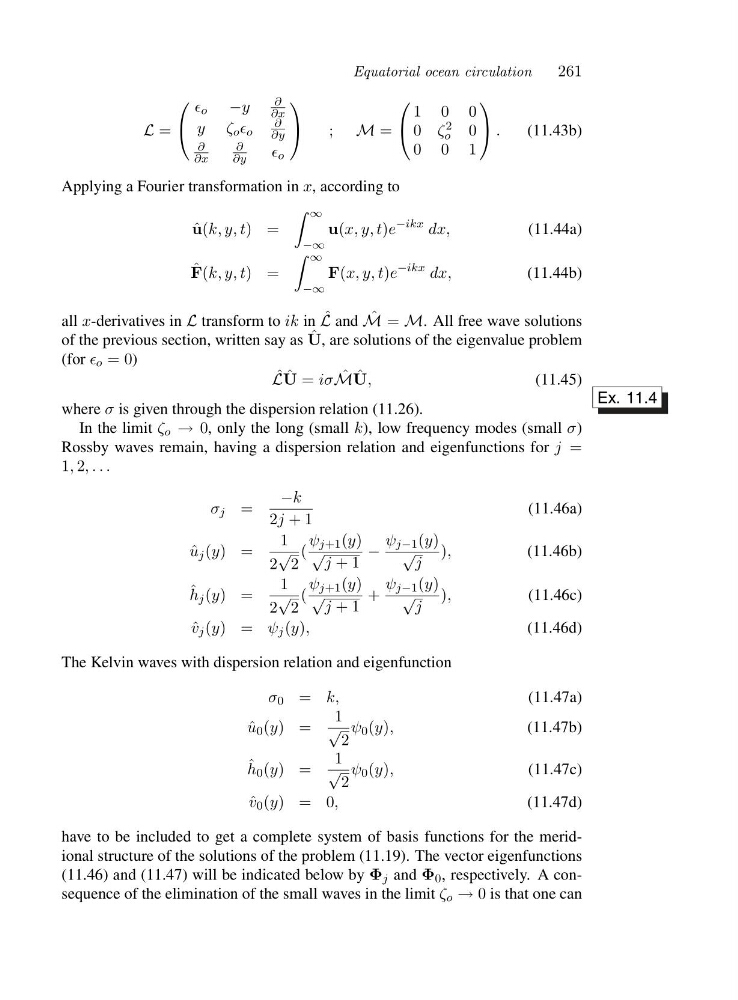
Applying a Fourier transformation in x, according to
ˆ
u(k, y, t)=
∞
−∞
u(x, y, t)e
−ikx dx,
(11.44a)
ˆ
F(k, y, t)=
∞
−∞
F(x, y, t)e
−ikx dx,
(11.44b)
all x-derivatives in L transform to ik in ˆ
L and ˆ
M = M. All free wave solutions
of the previous section, written say as ˆ
U, are solutions of the eigenvalue problem
(for ǫ o =0)
ˆ
L ˆ
U = iσ ˆ
M ˆ
U,
(11.45)
where σ is given through the dispersion relation (11.26).
Ex. 11.4
In the limit ζ o → 0, only the long (small k), low frequency modes (small σ)
Rossby waves remain, having a dispersion relation and eigenfunctions for j =
1, 2,...
σ j =
−k
2j +1
(11.46a)
ˆ
u j (y)=
1
2
√
2
(
ψ j+1 (y)
√ j +1
−
ψ j−1 (y)
√ j
),
(11.46b)
ˆ
h j (y)=
1
2
√
2
(
ψ j+1 (y)
√ j +1
+
ψ j−1 (y)
√ j
),
(11.46c)
ˆ
v j (y)=ψ j (y),
(11.46d)
The Kelvin waves with dispersion relation and eigenfunction
σ 0 = k,
(11.47a)
ˆ
u 0 (y)=
1
√
2
ψ 0 (y),
(11.47b)
ˆ
h 0 (y)=
1
√
2
ψ 0 (y),
(11.47c)
ˆ
v 0 (y)=0 ,
(11.47d)
have to be included to get a complete system of basis functions for the meridional structure of the solutions of the problem (11.19). The vector eigenfunctions
(11.46) and (11.47) will be indicated below by Φ j and Φ 0 , respectively. A consequence of the elimination of the small waves in the limit ζ o → 0 is that one can
261
L =
⎛
⎝
ǫ o −y
∂
∂x
yζ o ǫ o
∂
∂y
∂
∂x
∂
∂y
ǫ o
⎞
⎠
; M =
⎛
⎝
100
0 ζ 2
o
0
001
⎞
⎠ .
(11.43b)
Applying a Fourier transformation in x, according to
ˆ
u(k, y, t)=
∞
−∞
u(x, y, t)e
−ikx dx,
(11.44a)
ˆ
F(k, y, t)=
∞
−∞
F(x, y, t)e
−ikx dx,
(11.44b)
all x-derivatives in L transform to ik in ˆ
L and ˆ
M = M. All free wave solutions
of the previous section, written say as ˆ
U, are solutions of the eigenvalue problem
(for ǫ o =0)
ˆ
L ˆ
U = iσ ˆ
M ˆ
U,
(11.45)
where σ is given through the dispersion relation (11.26).
Ex. 11.4
In the limit ζ o → 0, only the long (small k), low frequency modes (small σ)
Rossby waves remain, having a dispersion relation and eigenfunctions for j =
1, 2,...
σ j =
−k
2j +1
(11.46a)
ˆ
u j (y)=
1
2
√
2
(
ψ j+1 (y)
√ j +1
−
ψ j−1 (y)
√ j
),
(11.46b)
ˆ
h j (y)=
1
2
√
2
(
ψ j+1 (y)
√ j +1
+
ψ j−1 (y)
√ j
),
(11.46c)
ˆ
v j (y)=ψ j (y),
(11.46d)
The Kelvin waves with dispersion relation and eigenfunction
σ 0 = k,
(11.47a)
ˆ
u 0 (y)=
1
√
2
ψ 0 (y),
(11.47b)
ˆ
h 0 (y)=
1
√
2
ψ 0 (y),
(11.47c)
ˆ
v 0 (y)=0 ,
(11.47d)
have to be included to get a complete system of basis functions for the meridional structure of the solutions of the problem (11.19). The vector eigenfunctions
(11.46) and (11.47) will be indicated below by Φ j and Φ 0 , respectively. A consequence of the elimination of the small waves in the limit ζ o → 0 is that one can