

260
DYNAMICAL OCEANOGRAPHY
Additional Material
B: Equatorial waves are discussed at length in section 8.5 of Pedlosky (1987),
the chapters 3 and 4 of Philander (1990) and lecture 18 of Pedlosky (2003).
11.5. Forced response in a basin
Using the reduced model derived in section 11.2, we next consider the changes
in the ocean circulation in a finite basin due to the presence of a prescribed wind
stress. Under limitations of small amplitude forced motion, the shallow water
model can be linearized around a motionless reference state with constant thermocline depth H. Small amplitude zonal winds are assumed to be present, while
the meridional component of the wind is neglected. A further simplification arises
by idealizing the horizontal friction to be linear rather than harmonic. This can be
justified by recognizing that for equatorially trapped motions in which the zonal
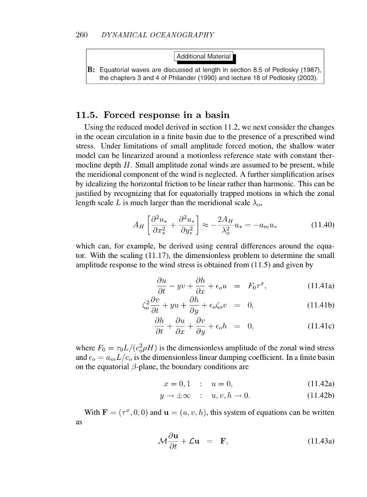
length scale L is much larger than the meridional scale λ o ,
A H
∂ 2 u ∗
∂x 2
∗
+
∂ 2 u ∗
∂y 2
∗
≈−
2A H
λ 2
o
u ∗ = −a m u ∗
(11.40)
which can, for example, be derived using central differences around the equator. With the scaling (11.17), the dimensionless problem to determine the small
amplitude response to the wind stress is obtained from (11.5) and given by
∂u
∂t
− yv +
∂h
∂x
+ ǫ o u = F 0 τ
x ,
(11.41a)
ζ
2
o
∂v
∂t
+ yu +
∂h
∂y
+ ǫ o ζ o v =0 ,
(11.41b)
∂h
∂t
+
∂u
∂x
+
∂v
∂y
+ ǫ o h =0 ,
(11.41c)
where F 0 = τ 0 L/(c 2
o ρH) is the dimensionless amplitude of the zonal wind stress
and ǫ o = a m L/c o is the dimensionless linear damping coefficient. In a finite basin
on the equatorial β-plane, the boundary conditions are
x =0, 1:u =0,
(11.42a)
y →±∞ : u, v, h → 0.
(11.42b)
With F =(τ x , 0, 0) and u =(u, v, h), this system of equations can be written
as
M
∂u
∂t
+ Lu = F,
(11.43a)
DYNAMICAL OCEANOGRAPHY
Additional Material
B: Equatorial waves are discussed at length in section 8.5 of Pedlosky (1987),
the chapters 3 and 4 of Philander (1990) and lecture 18 of Pedlosky (2003).
11.5. Forced response in a basin
Using the reduced model derived in section 11.2, we next consider the changes
in the ocean circulation in a finite basin due to the presence of a prescribed wind
stress. Under limitations of small amplitude forced motion, the shallow water
model can be linearized around a motionless reference state with constant thermocline depth H. Small amplitude zonal winds are assumed to be present, while
the meridional component of the wind is neglected. A further simplification arises
by idealizing the horizontal friction to be linear rather than harmonic. This can be
justified by recognizing that for equatorially trapped motions in which the zonal
length scale L is much larger than the meridional scale λ o ,
A H
∂ 2 u ∗
∂x 2
∗
+
∂ 2 u ∗
∂y 2
∗
≈−
2A H
λ 2
o
u ∗ = −a m u ∗
(11.40)
which can, for example, be derived using central differences around the equator. With the scaling (11.17), the dimensionless problem to determine the small
amplitude response to the wind stress is obtained from (11.5) and given by
∂u
∂t
− yv +
∂h
∂x
+ ǫ o u = F 0 τ
x ,
(11.41a)
ζ
2
o
∂v
∂t
+ yu +
∂h
∂y
+ ǫ o ζ o v =0 ,
(11.41b)
∂h
∂t
+
∂u
∂x
+
∂v
∂y
+ ǫ o h =0 ,
(11.41c)
where F 0 = τ 0 L/(c 2
o ρH) is the dimensionless amplitude of the zonal wind stress
and ǫ o = a m L/c o is the dimensionless linear damping coefficient. In a finite basin
on the equatorial β-plane, the boundary conditions are
x =0, 1:u =0,
(11.42a)
y →±∞ : u, v, h → 0.
(11.42b)
With F =(τ x , 0, 0) and u =(u, v, h), this system of equations can be written
as
M
∂u
∂t
+ Lu = F,
(11.43a)