

250
DYNAMICAL OCEANOGRAPHY
where ¯
E V =2 A V /(β 0 L 3 )=2 E V , where E V is the equatorial vertical Ekman
number; horizontal mixing is neglected.
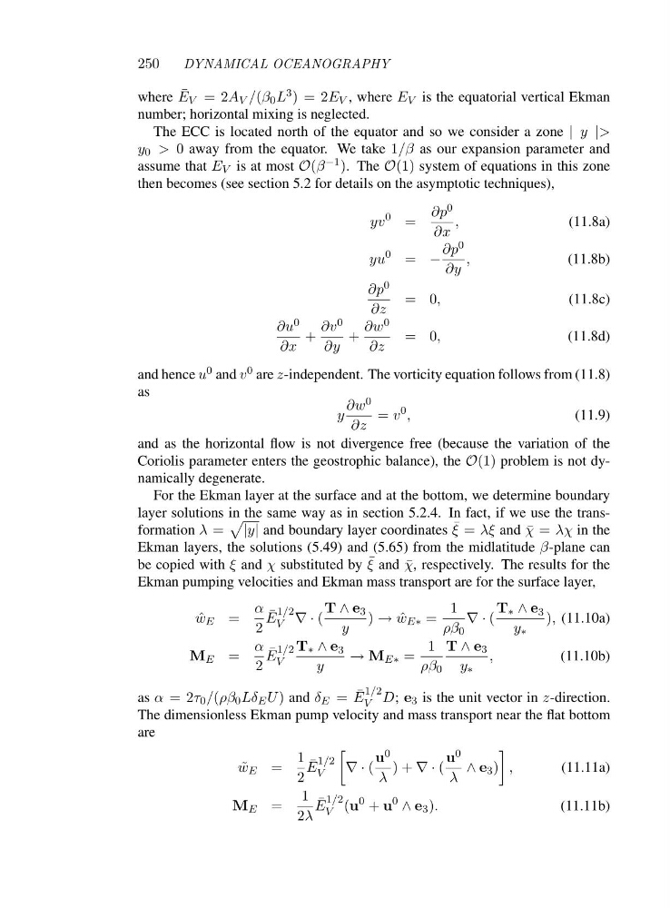
The ECC is located north of the equator and so we consider a zone | y |>
y 0 > 0 away from the equator. We take 1/β as our expansion parameter and
assume that E V is at most O(β −1 ).T h eO(1) system of equations in this zone
then becomes (see section 5.2 for details on the asymptotic techniques),
yv
0 =
∂p 0
∂x
,
(11.8a)
yu
0 = −
∂p 0
∂y
,
(11.8b)
∂p 0
∂z
=0 ,
(11.8c)
∂u 0
∂x
+
∂v 0
∂y
+
∂w 0
∂z
=0 ,
(11.8d)
and hence u 0 and v 0 are z-independent. The vorticity equation follows from (11.8)
as
y
∂w 0
∂z
= v
0 ,
(11.9)
and as the horizontal flow is not divergence free (because the variation of the
Coriolis parameter enters the geostrophic balance), the O(1) problem is not dynamically degenerate.
For the Ekman layer at the surface and at the bottom, we determine boundary
layer solutions in the same way as in section 5.2.4. In fact, if we use the transformation λ =
|y| and boundary layer coordinates ¯
ξ = λξ and ¯
χ = λχ in the
Ekman layers, the solutions (5.49) and (5.65) from the midlatitude β-plane can
be copied with ξ and χ substituted by ¯
ξ and ¯
χ, respectively. The results for the
Ekman pumping velocities and Ekman mass transport are for the surface layer,
ˆ
w E =
α
2
¯
E
1/2
V ∇·(
T ∧ e 3
y
) → ˆ
w E∗ =
1
ρβ 0
∇·(
T ∗ ∧ e 3
y ∗
), (11.10a)
M E =
α
2
¯
E
1/2
V
T ∗ ∧ e 3
y
→ M E∗ =
1
ρβ 0
T ∧ e 3
y ∗
,
(11.10b)
as α =2 τ 0 /(ρβ 0 Lδ E U ) and δ E = ¯
E
1/2
V D; e 3 is the unit vector in z-direction.
The dimensionless Ekman pump velocity and mass transport near the flat bottom
are
˜
w E =
1
2
¯
E
1/2
V
∇·(
u 0
λ
)+∇·(
u 0
λ
∧ e 3 )
,
(11.11a)
M E =
1
2λ
¯
E
1/2
V (u
0 + u
0 ∧ e 3 ).
(11.11b)
DYNAMICAL OCEANOGRAPHY
where ¯
E V =2 A V /(β 0 L 3 )=2 E V , where E V is the equatorial vertical Ekman
number; horizontal mixing is neglected.
The ECC is located north of the equator and so we consider a zone | y |>
y 0 > 0 away from the equator. We take 1/β as our expansion parameter and
assume that E V is at most O(β −1 ).T h eO(1) system of equations in this zone
then becomes (see section 5.2 for details on the asymptotic techniques),
yv
0 =
∂p 0
∂x
,
(11.8a)
yu
0 = −
∂p 0
∂y
,
(11.8b)
∂p 0
∂z
=0 ,
(11.8c)
∂u 0
∂x
+
∂v 0
∂y
+
∂w 0
∂z
=0 ,
(11.8d)
and hence u 0 and v 0 are z-independent. The vorticity equation follows from (11.8)
as
y
∂w 0
∂z
= v
0 ,
(11.9)
and as the horizontal flow is not divergence free (because the variation of the
Coriolis parameter enters the geostrophic balance), the O(1) problem is not dynamically degenerate.
For the Ekman layer at the surface and at the bottom, we determine boundary
layer solutions in the same way as in section 5.2.4. In fact, if we use the transformation λ =
|y| and boundary layer coordinates ¯
ξ = λξ and ¯
χ = λχ in the
Ekman layers, the solutions (5.49) and (5.65) from the midlatitude β-plane can
be copied with ξ and χ substituted by ¯
ξ and ¯
χ, respectively. The results for the
Ekman pumping velocities and Ekman mass transport are for the surface layer,
ˆ
w E =
α
2
¯
E
1/2
V ∇·(
T ∧ e 3
y
) → ˆ
w E∗ =
1
ρβ 0
∇·(
T ∗ ∧ e 3
y ∗
), (11.10a)
M E =
α
2
¯
E
1/2
V
T ∗ ∧ e 3
y
→ M E∗ =
1
ρβ 0
T ∧ e 3
y ∗
,
(11.10b)
as α =2 τ 0 /(ρβ 0 Lδ E U ) and δ E = ¯
E
1/2
V D; e 3 is the unit vector in z-direction.
The dimensionless Ekman pump velocity and mass transport near the flat bottom
are
˜
w E =
1
2
¯
E
1/2
V
∇·(
u 0
λ
)+∇·(
u 0
λ
∧ e 3 )
,
(11.11a)
M E =
1
2λ
¯
E
1/2
V (u
0 + u
0 ∧ e 3 ).
(11.11b)