

Equatorial ocean circulation
251
The vorticity equation follows directly from (11.9) through integration over the
layer as
y
2
E
1/2
V
α∇·(y
−1 T ∧ e 3 ) −∇·(
u 0
λ
) −∇·(
u 0
λ
∧ e 3 )
= v
0 .
(11.12)
If we choose U such that α ¯
E
1/2
V
=2 , i.e., U = τ 0 /(ρβ 0 LD) then the Sverdrup
balance becomes
v
0 = y∇·(y
−1 T ∧ e 3 )=
∂τ y
∂x
−
∂τ x
∂y
+
τ x
y
.
(11.13)
With L =1 0 6 and D =1 0 3 we find U ≈ 10 −2 ms −1 if τ 0 =1 0 −1 Nm −2 ;t h i s
velocity should again be seen as a depth averaged velocity.
◮
Example 11.1: Idealized model of the ECC
As an example we consider an idealization of the equatorial wind-stress field
as
τ
x (y)=−
1
2
(1 + cos 2π(y − y 0 )),
(11.14)
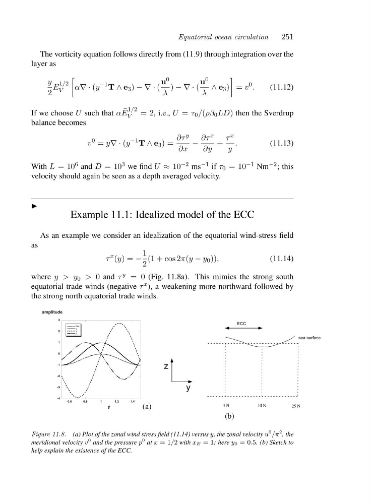
where y>y 0 > 0 and τ y =0(Fig. 11.8a). This mimics the strong south
equatorial trade winds (negative τ x ), a weakening more northward followed by
the strong north equatorial trade winds.
-4
-3
-2
-1
0
1
2
3
0.6
0.8
1
1.2
1.4
tau
u
v
p
amplitude
y
(a)
y
4 Ν
10 Ν
z
25 Ν
sea surface
ECC
(b)
Figure 11.8. (a) Plot of the zonal wind stress field (11.14) versus y, the zonal velocity u
0 /π
2 ,the
meridional velocity v
0 and the pressure p
0 at x =1 /2 with xE =1 ;her ey0 =0 .5. (b) Sketch to
help explain the existence of the ECC.
251
The vorticity equation follows directly from (11.9) through integration over the
layer as
y
2
E
1/2
V
α∇·(y
−1 T ∧ e 3 ) −∇·(
u 0
λ
) −∇·(
u 0
λ
∧ e 3 )
= v
0 .
(11.12)
If we choose U such that α ¯
E
1/2
V
=2 , i.e., U = τ 0 /(ρβ 0 LD) then the Sverdrup
balance becomes
v
0 = y∇·(y
−1 T ∧ e 3 )=
∂τ y
∂x
−
∂τ x
∂y
+
τ x
y
.
(11.13)
With L =1 0 6 and D =1 0 3 we find U ≈ 10 −2 ms −1 if τ 0 =1 0 −1 Nm −2 ;t h i s
velocity should again be seen as a depth averaged velocity.
◮
Example 11.1: Idealized model of the ECC
As an example we consider an idealization of the equatorial wind-stress field
as
τ
x (y)=−
1
2
(1 + cos 2π(y − y 0 )),
(11.14)
where y>y 0 > 0 and τ y =0(Fig. 11.8a). This mimics the strong south
equatorial trade winds (negative τ x ), a weakening more northward followed by
the strong north equatorial trade winds.
-4
-3
-2
-1
0
1
2
3
0.6
0.8
1
1.2
1.4
tau
u
v
p
amplitude
y
(a)
y
4 Ν
10 Ν
z
25 Ν
sea surface
ECC
(b)
Figure 11.8. (a) Plot of the zonal wind stress field (11.14) versus y, the zonal velocity u
0 /π
2 ,the
meridional velocity v
0 and the pressure p
0 at x =1 /2 with xE =1 ;her ey0 =0 .5. (b) Sketch to
help explain the existence of the ECC.