

Equatorial ocean circulation
249
D
dt ∗
(z ∗ + H − ζ ∗ )=0 ,
(11.4b)
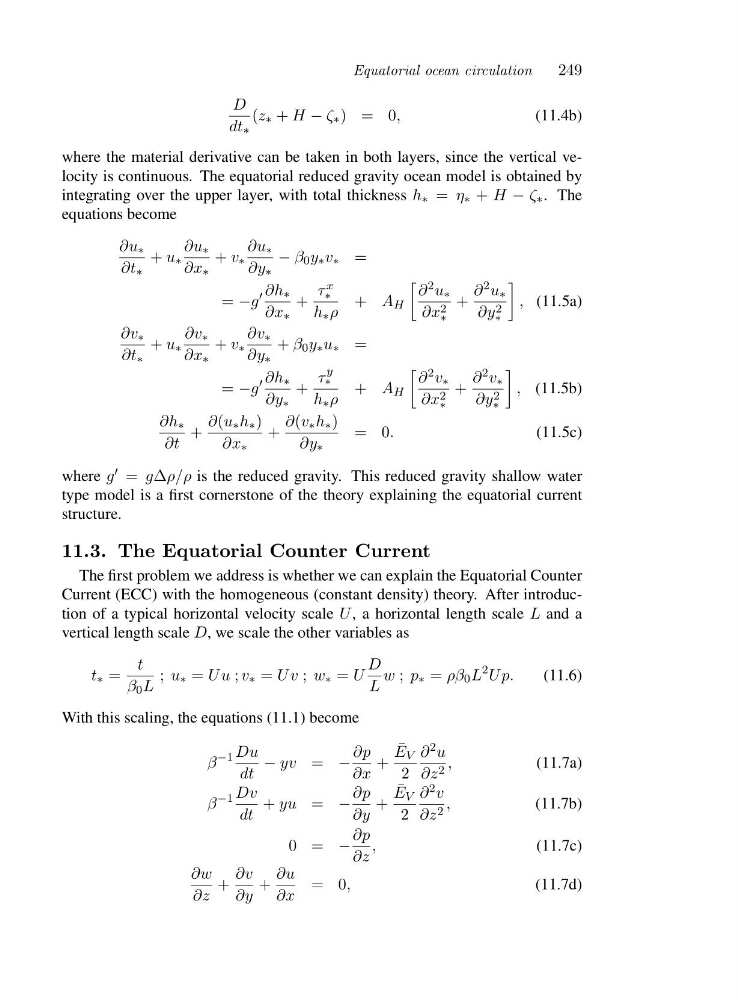
where the material derivative can be taken in both layers, since the vertical velocity is continuous. The equatorial reduced gravity ocean model is obtained by
integrating over the upper layer, with total thickness h ∗ = η ∗ + H − ζ ∗ .T h e
equations become
∂u ∗
∂t ∗
+ u ∗
∂u ∗
∂x ∗
+ v ∗
∂u ∗
∂y ∗
− β 0 y ∗ v ∗ =
= −g
′ ∂h ∗
∂x ∗
+
τ x
∗
h ∗ ρ
+ A H
∂ 2 u ∗
∂x 2
∗
+
∂ 2 u ∗
∂y 2
∗
, (11.5a)
∂v ∗
∂t ∗
+ u ∗
∂v ∗
∂x ∗
+ v ∗
∂v ∗
∂y ∗
+ β 0 y ∗ u ∗ =
= −g
′ ∂h ∗
∂y ∗
+
τ
y
∗
h ∗ ρ
+ A H
∂ 2 v ∗
∂x 2
∗
+
∂ 2 v ∗
∂y 2
∗
, (11.5b)
∂h ∗
∂t
+
∂(u ∗ h ∗ )
∂x ∗
+
∂(v ∗ h ∗ )
∂y ∗
=0 .
(11.5c)
where g ′ = gΔρ/ρ is the reduced gravity. This reduced gravity shallow water
type model is a first cornerstone of the theory explaining the equatorial current
structure.
11.3. The Equatorial Counter Current
The first problem we address is whether we can explain the Equatorial Counter
Current (ECC) with the homogeneous (constant density) theory. After introduction of a typical horizontal velocity scale U , a horizontal length scale L and a
vertical length scale D, we scale the other variables as
t ∗ =
t
β 0 L
; u ∗ = Uu ; v ∗ = Uv ; w ∗ = U
D
L
w ; p ∗ = ρβ 0 L
2 Up.
(11.6)
With this scaling, the equations (11.1) become
β
−1 Du
dt
− yv = −
∂p
∂x
+
¯
E V
2
∂ 2 u
∂z 2 ,
(11.7a)
β
−1 Dv
dt
+ yu = −
∂p
∂y
+
¯
E V
2
∂ 2 v
∂z 2 ,
(11.7b)
0=−
∂p
∂z
,
(11.7c)
∂w
∂z
+
∂v
∂y
+
∂u
∂x
=0 ,
(11.7d)
249
D
dt ∗
(z ∗ + H − ζ ∗ )=0 ,
(11.4b)
where the material derivative can be taken in both layers, since the vertical velocity is continuous. The equatorial reduced gravity ocean model is obtained by
integrating over the upper layer, with total thickness h ∗ = η ∗ + H − ζ ∗ .T h e
equations become
∂u ∗
∂t ∗
+ u ∗
∂u ∗
∂x ∗
+ v ∗
∂u ∗
∂y ∗
− β 0 y ∗ v ∗ =
= −g
′ ∂h ∗
∂x ∗
+
τ x
∗
h ∗ ρ
+ A H
∂ 2 u ∗
∂x 2
∗
+
∂ 2 u ∗
∂y 2
∗
, (11.5a)
∂v ∗
∂t ∗
+ u ∗
∂v ∗
∂x ∗
+ v ∗
∂v ∗
∂y ∗
+ β 0 y ∗ u ∗ =
= −g
′ ∂h ∗
∂y ∗
+
τ
y
∗
h ∗ ρ
+ A H
∂ 2 v ∗
∂x 2
∗
+
∂ 2 v ∗
∂y 2
∗
, (11.5b)
∂h ∗
∂t
+
∂(u ∗ h ∗ )
∂x ∗
+
∂(v ∗ h ∗ )
∂y ∗
=0 .
(11.5c)
where g ′ = gΔρ/ρ is the reduced gravity. This reduced gravity shallow water
type model is a first cornerstone of the theory explaining the equatorial current
structure.
11.3. The Equatorial Counter Current
The first problem we address is whether we can explain the Equatorial Counter
Current (ECC) with the homogeneous (constant density) theory. After introduction of a typical horizontal velocity scale U , a horizontal length scale L and a
vertical length scale D, we scale the other variables as
t ∗ =
t
β 0 L
; u ∗ = Uu ; v ∗ = Uv ; w ∗ = U
D
L
w ; p ∗ = ρβ 0 L
2 Up.
(11.6)
With this scaling, the equations (11.1) become
β
−1 Du
dt
− yv = −
∂p
∂x
+
¯
E V
2
∂ 2 u
∂z 2 ,
(11.7a)
β
−1 Dv
dt
+ yu = −
∂p
∂y
+
¯
E V
2
∂ 2 v
∂z 2 ,
(11.7b)
0=−
∂p
∂z
,
(11.7c)
∂w
∂z
+
∂v
∂y
+
∂u
∂x
=0 ,
(11.7d)