

248
DYNAMICAL OCEANOGRAPHY
ρA V
∂v ∗
∂z ∗
= τ
y
∗ ,
(11.2c)
D
dt ∗
(z ∗ − η ∗ )=0.
(11.2d)
In these equations, u ∗ and v ∗ are the horizontal velocities, w ∗ is the vertical
velocity and p ∗ is the pressure. The quantities g, A H ,andA V are the acceleration
due to gravity and the horizontal and vertical mixing coefficients of momentum.
The quantity p a∗ is the background atmospheric sea level pressure and (τ x
∗ ,τ
y
∗ ) is
the wind-stress forcing. Other boundary conditions for the flow, for example at
the continental boundaries, will be specified later.
11.2.2. The reduced gravity model
A slight extension of the previous model is the flow in a two-layer ocean in
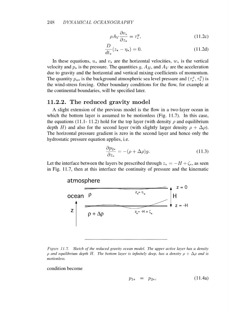
which the bottom layer is assumed to be motionless (Fig. 11.7). In this case,
the equations (11.1- 11.2) hold for the top layer (with density ρ and equilibrium
depth H) and also for the second layer (with slightly larger density ρ +Δ ρ).
The horizontal pressure gradient is zero in the second layer and hence only the
hydrostatic pressure equation applies, i.e.
∂p 2∗
∂z ∗
= −(ρ +Δρ)g.
(11.3)
Let the interface between the layers be prescribed through z ∗ = −H + ζ ∗ , as seen
in Fig. 11.7, then at this interface the continuity of pressure and the kinematic
atmosphere
ρ
ρ + Δρ
H
z = -H + ζ
z = η
*
*
*
*
ocean
z
z = 0
z = -H
Figure 11.7. Sketch of the reduced gravity ocean model. The upper active layer has a density
ρ and equilibrium depth H. The bottom layer is infinitely deep, has a density ρ +∆ ρ and is
motionless.
condition become
p 1∗ = p 2∗ ,
(11.4a)
DYNAMICAL OCEANOGRAPHY
ρA V
∂v ∗
∂z ∗
= τ
y
∗ ,
(11.2c)
D
dt ∗
(z ∗ − η ∗ )=0.
(11.2d)
In these equations, u ∗ and v ∗ are the horizontal velocities, w ∗ is the vertical
velocity and p ∗ is the pressure. The quantities g, A H ,andA V are the acceleration
due to gravity and the horizontal and vertical mixing coefficients of momentum.
The quantity p a∗ is the background atmospheric sea level pressure and (τ x
∗ ,τ
y
∗ ) is
the wind-stress forcing. Other boundary conditions for the flow, for example at
the continental boundaries, will be specified later.
11.2.2. The reduced gravity model
A slight extension of the previous model is the flow in a two-layer ocean in
which the bottom layer is assumed to be motionless (Fig. 11.7). In this case,
the equations (11.1- 11.2) hold for the top layer (with density ρ and equilibrium
depth H) and also for the second layer (with slightly larger density ρ +Δ ρ).
The horizontal pressure gradient is zero in the second layer and hence only the
hydrostatic pressure equation applies, i.e.
∂p 2∗
∂z ∗
= −(ρ +Δρ)g.
(11.3)
Let the interface between the layers be prescribed through z ∗ = −H + ζ ∗ , as seen
in Fig. 11.7, then at this interface the continuity of pressure and the kinematic
atmosphere
ρ
ρ + Δρ
H
z = -H + ζ
z = η
*
*
*
*
ocean
z
z = 0
z = -H
Figure 11.7. Sketch of the reduced gravity ocean model. The upper active layer has a density
ρ and equilibrium depth H. The bottom layer is infinitely deep, has a density ρ +∆ ρ and is
motionless.
condition become
p 1∗ = p 2∗ ,
(11.4a)