

228
DYNAMICAL OCEANOGRAPHY
-0.2
0
0.2
0.4
0.6
012345
k
kc
i
S = 0.25
S = 0.5
S = 1.0
S = 2.0
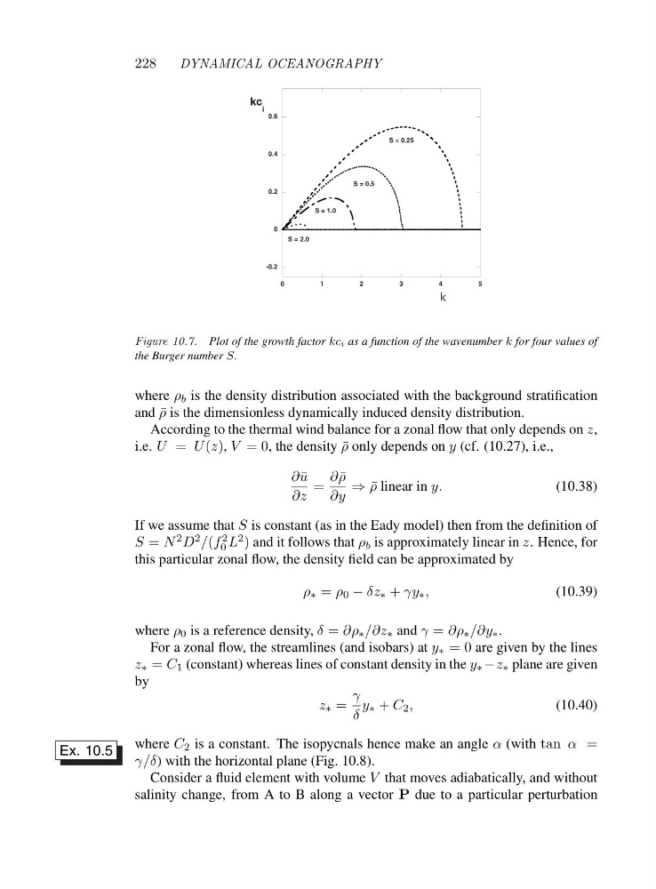
Figure 10.7. Plot of the growth factor kci as a function of the wavenumber k for four values of
the Burger number S.
where ρ b is the density distribution associated with the background stratification
and ¯
ρ is the dimensionless dynamically induced density distribution.
According to the thermal wind balance for a zonal flow that only depends on z,
i.e. U = U (z), V =0, the density ¯
ρ only depends on y (cf. (10.27), i.e.,
∂ ¯
u
∂z
=
∂ ¯
ρ
∂y
⇒ ¯
ρ linear in y.
(10.38)
If we assume that S is constant (as in the Eady model) then from the definition of
S = N 2 D 2 /(f 2
0 L 2 ) and it follows that ρ b is approximately linear in z. Hence, for
this particular zonal flow, the density field can be approximated by
ρ ∗ = ρ 0 − δz ∗ + γy ∗ ,
(10.39)
where ρ 0 is a reference density, δ = ∂ρ ∗ /∂z ∗ and γ = ∂ρ ∗ /∂y ∗ .
For a zonal flow, the streamlines (and isobars) at y ∗ =0are given by the lines
z ∗ = C 1 (constant) whereas lines of constant density in the y ∗ −z ∗ plane are given
by
z ∗ =
γ
δ
y ∗ + C 2 ,
(10.40)
where C 2 is a constant. The isopycnals hence make an angle α (with tan α =
γ/δ) with the horizontal plane (Fig. 10.8).
Ex. 10.5
Consider a fluid element with volume V that moves adiabatically, and without
salinity change, from A to B along a vector P due to a particular perturbation
DYNAMICAL OCEANOGRAPHY
-0.2
0
0.2
0.4
0.6
012345
k
kc
i
S = 0.25
S = 0.5
S = 1.0
S = 2.0
Figure 10.7. Plot of the growth factor kci as a function of the wavenumber k for four values of
the Burger number S.
where ρ b is the density distribution associated with the background stratification
and ¯
ρ is the dimensionless dynamically induced density distribution.
According to the thermal wind balance for a zonal flow that only depends on z,
i.e. U = U (z), V =0, the density ¯
ρ only depends on y (cf. (10.27), i.e.,
∂ ¯
u
∂z
=
∂ ¯
ρ
∂y
⇒ ¯
ρ linear in y.
(10.38)
If we assume that S is constant (as in the Eady model) then from the definition of
S = N 2 D 2 /(f 2
0 L 2 ) and it follows that ρ b is approximately linear in z. Hence, for
this particular zonal flow, the density field can be approximated by
ρ ∗ = ρ 0 − δz ∗ + γy ∗ ,
(10.39)
where ρ 0 is a reference density, δ = ∂ρ ∗ /∂z ∗ and γ = ∂ρ ∗ /∂y ∗ .
For a zonal flow, the streamlines (and isobars) at y ∗ =0are given by the lines
z ∗ = C 1 (constant) whereas lines of constant density in the y ∗ −z ∗ plane are given
by
z ∗ =
γ
δ
y ∗ + C 2 ,
(10.40)
where C 2 is a constant. The isopycnals hence make an angle α (with tan α =
γ/δ) with the horizontal plane (Fig. 10.8).
Ex. 10.5
Consider a fluid element with volume V that moves adiabatically, and without
salinity change, from A to B along a vector P due to a particular perturbation