

Stability of zonal flows
227
0
0.2
0.4
0.6
0.8
1
0
0.5
1
1.5
2
2.5
3
µ µ
µ
µ
c
i
(a)
-1
-0.5
0
0.5
1
012345678
µ µ µ
µ
c
r
(b)
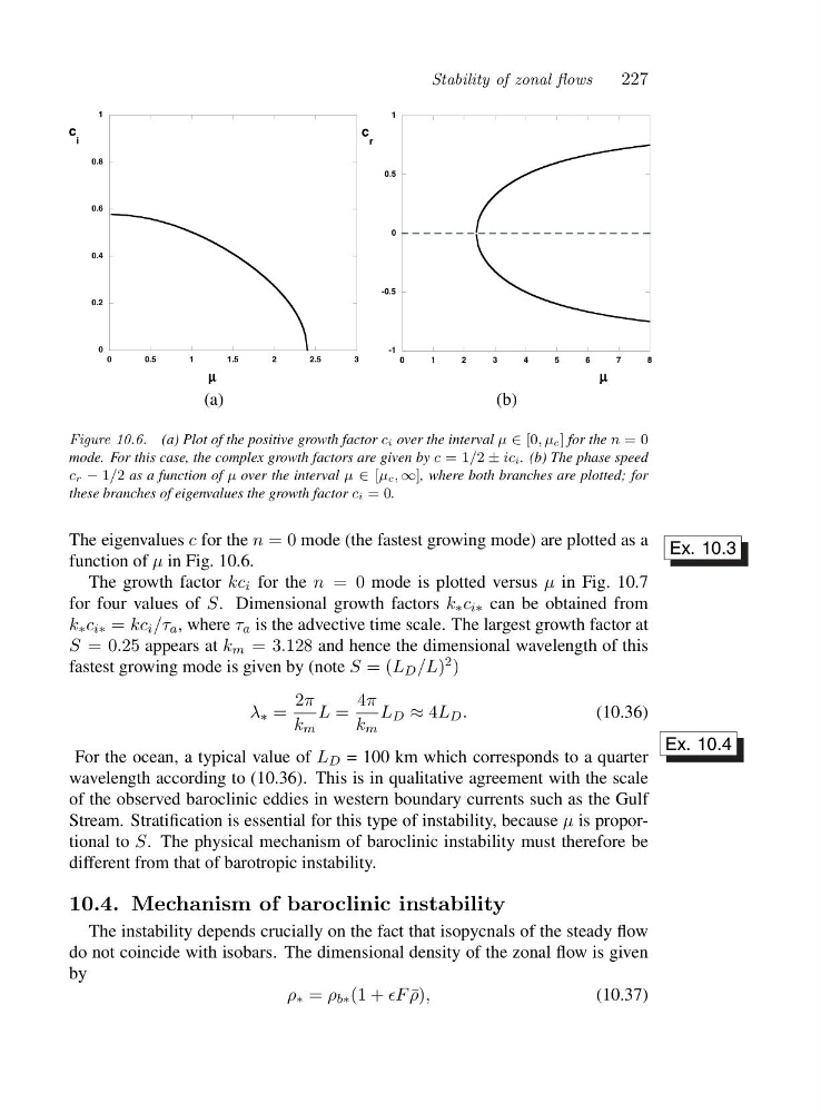
Figure 10.6. (a) Plot of the positive growth factor ci over the interval μ ∈ [0,μc] for the n =0
mode. For this case, the complex growth factors are given by c =1 /2 ± ici. (b) The phase speed
cr − 1/2 as a function of μ over the interval μ ∈ [μc, ∞], where both branches are plotted; for
these branches of eigenvalues the growth factor ci =0.
The eigenvalues c for the n =0mode (the fastest growing mode) are plotted as a
function of μ in Fig. 10.6.
Ex. 10.3
The growth factor kc i for the n =0mode is plotted versus μ in Fig. 10.7
for four values of S. Dimensional growth factors k ∗ c i∗ can be obtained from
k ∗ c i∗ = kc i /τ a , where τ a is the advective time scale. The largest growth factor at
S =0 .25 appears at k m =3 .128 and hence the dimensional wavelength of this
fastest growing mode is given by (note S =(L D /L) 2 )
λ ∗ =
2π
k m
L =
4π
k m
L D ≈ 4L D .
(10.36)
For the ocean, a typical value of L D = 100 km which corresponds to a quarter
Ex. 10.4
wavelength according to (10.36). This is in qualitative agreement with the scale
of the observed baroclinic eddies in western boundary currents such as the Gulf
Stream. Stratification is essential for this type of instability, because μ is proportional to S. The physical mechanism of baroclinic instability must therefore be
different from that of barotropic instability.
10.4. Mechanism of baroclinic instability
The instability depends crucially on the fact that isopycnals of the steady flow
do not coincide with isobars. The dimensional density of the zonal flow is given
by
ρ ∗ = ρ b∗ (1 + ǫF ¯
ρ),
(10.37)
227
0
0.2
0.4
0.6
0.8
1
0
0.5
1
1.5
2
2.5
3
µ µ
µ
µ
c
i
(a)
-1
-0.5
0
0.5
1
012345678
µ µ µ
µ
c
r
(b)
Figure 10.6. (a) Plot of the positive growth factor ci over the interval μ ∈ [0,μc] for the n =0
mode. For this case, the complex growth factors are given by c =1 /2 ± ici. (b) The phase speed
cr − 1/2 as a function of μ over the interval μ ∈ [μc, ∞], where both branches are plotted; for
these branches of eigenvalues the growth factor ci =0.
The eigenvalues c for the n =0mode (the fastest growing mode) are plotted as a
function of μ in Fig. 10.6.
Ex. 10.3
The growth factor kc i for the n =0mode is plotted versus μ in Fig. 10.7
for four values of S. Dimensional growth factors k ∗ c i∗ can be obtained from
k ∗ c i∗ = kc i /τ a , where τ a is the advective time scale. The largest growth factor at
S =0 .25 appears at k m =3 .128 and hence the dimensional wavelength of this
fastest growing mode is given by (note S =(L D /L) 2 )
λ ∗ =
2π
k m
L =
4π
k m
L D ≈ 4L D .
(10.36)
For the ocean, a typical value of L D = 100 km which corresponds to a quarter
Ex. 10.4
wavelength according to (10.36). This is in qualitative agreement with the scale
of the observed baroclinic eddies in western boundary currents such as the Gulf
Stream. Stratification is essential for this type of instability, because μ is proportional to S. The physical mechanism of baroclinic instability must therefore be
different from that of barotropic instability.
10.4. Mechanism of baroclinic instability
The instability depends crucially on the fact that isopycnals of the steady flow
do not coincide with isobars. The dimensional density of the zonal flow is given
by
ρ ∗ = ρ b∗ (1 + ǫF ¯
ρ),
(10.37)