

226
DYNAMICAL OCEANOGRAPHY
and the eigenvalue problem for the eigenvalue c becomes
A
′′ − μ
2 A =0 ,
(10.32a)
(1 − c)A
′ (0) − A(0) = 0,
(10.32b)
cA
′ (−1) + A(−1) = 0,
(10.32c)
with μ 2 =(k 2 +[(n +
1
2 )π] 2 )S. The solution of (10.32a) is
A(z)=C 1 e
μz + C 2 e
−μz .
(10.33)
Substitution of this solution into the homogeneous equations (10.32b-c) and setting the coefficient determinant to zero provides the eigenvalues c.W efi n d
c =
1
2
±
1
μ
(
μ
2
−
1
tanh
μ
2
)(
μ
2
− tanh
μ
2
)
1/2
.
(10.34)
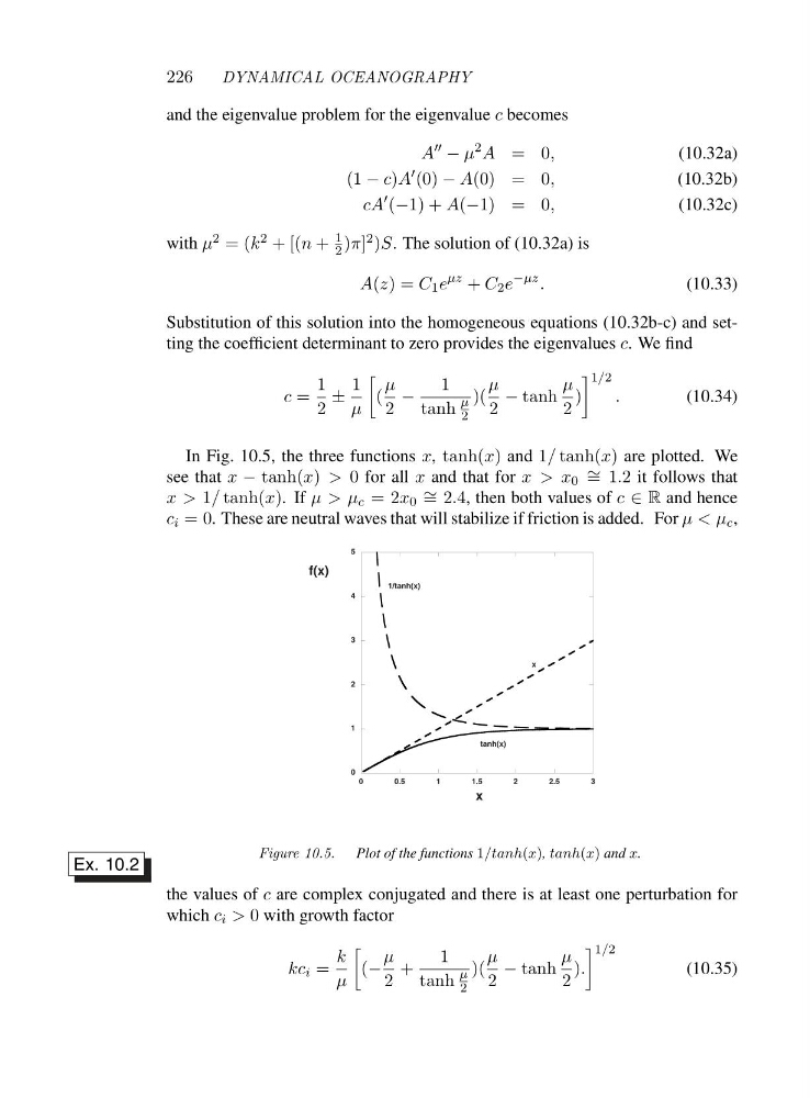
In Fig. 10.5, the three functions x, tanh(x) and 1/ tanh(x) are plotted. We
see that x − tanh(x) > 0 for all x and that for x>x 0 ∼ = 1.2 it follows that
x>1/ tanh(x).I fμ>μ c =2 x 0 ∼ = 2.4, then both values of c ∈ R and hence
c i =0. These are neutral waves that will stabilize if friction is added. For μ<μ c ,
0
1
2
3
4
5
0
0.5
1
1.5
2
2.5
3
x
f(x)
1/tanh(x)
tanh(x)
x
Figure 10.5. Plot of the functions 1/tanh(x), tanh(x) and x.
Ex. 10.2
the values of c are complex conjugated and there is at least one perturbation for
which c i > 0 with growth factor
kc i =
k
μ
(−
μ
2
+
1
tanh
μ
2
)(
μ
2
− tanh
μ
2
).
1/2
(10.35)
DYNAMICAL OCEANOGRAPHY
and the eigenvalue problem for the eigenvalue c becomes
A
′′ − μ
2 A =0 ,
(10.32a)
(1 − c)A
′ (0) − A(0) = 0,
(10.32b)
cA
′ (−1) + A(−1) = 0,
(10.32c)
with μ 2 =(k 2 +[(n +
1
2 )π] 2 )S. The solution of (10.32a) is
A(z)=C 1 e
μz + C 2 e
−μz .
(10.33)
Substitution of this solution into the homogeneous equations (10.32b-c) and setting the coefficient determinant to zero provides the eigenvalues c.W efi n d
c =
1
2
±
1
μ
(
μ
2
−
1
tanh
μ
2
)(
μ
2
− tanh
μ
2
)
1/2
.
(10.34)
In Fig. 10.5, the three functions x, tanh(x) and 1/ tanh(x) are plotted. We
see that x − tanh(x) > 0 for all x and that for x>x 0 ∼ = 1.2 it follows that
x>1/ tanh(x).I fμ>μ c =2 x 0 ∼ = 2.4, then both values of c ∈ R and hence
c i =0. These are neutral waves that will stabilize if friction is added. For μ<μ c ,
0
1
2
3
4
5
0
0.5
1
1.5
2
2.5
3
x
f(x)
1/tanh(x)
tanh(x)
x
Figure 10.5. Plot of the functions 1/tanh(x), tanh(x) and x.
Ex. 10.2
the values of c are complex conjugated and there is at least one perturbation for
which c i > 0 with growth factor
kc i =
k
μ
(−
μ
2
+
1
tanh
μ
2
)(
μ
2
− tanh
μ
2
).
1/2
(10.35)