

200
DYNAMICAL OCEANOGRAPHY
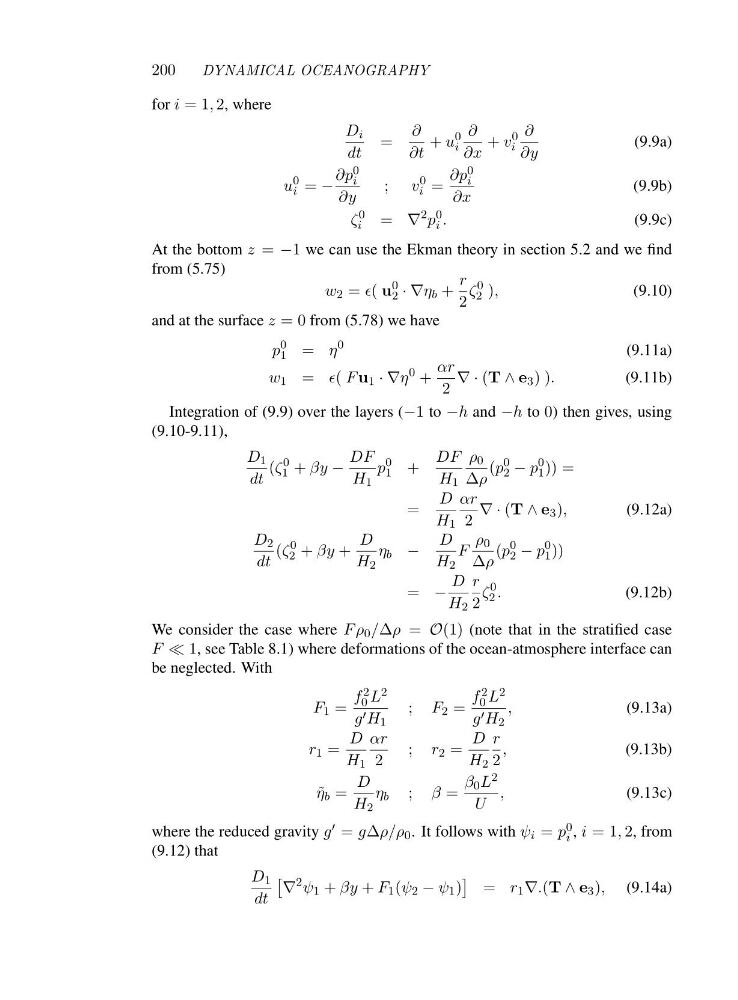
for i =1, 2, where
D i
dt
=
∂
∂t
+ u
0
i
∂
∂x
+ v
0
i
∂
∂y
(9.9a)
u
0
i = −
∂p 0
i
∂y
; v
0
i =
∂p 0
i
∂x
(9.9b)
ζ
0
i
= ∇
2 p
0
i .
(9.9c)
At the bottom z = −1 we can use the Ekman theory in section 5.2 and we find
from (5.75)
w 2 = ǫ( u
0
2 ·∇η b +
r
2
ζ
0
2 ),
(9.10)
and at the surface z =0from (5.78) we have
p
0
1 = η
0
(9.11a)
w 1 = ǫ( F u 1 ·∇η
0 +
αr
2
∇·(T ∧ e 3 )).
(9.11b)
Integration of (9.9) over the layers (−1 to −h and −h to 0) then gives, using
(9.10-9.11),
D 1
dt
(ζ
0
1 + βy −
DF
H 1
p
0
1 +
DF
H 1
ρ 0
Δρ
(p
0
2 − p
0
1 )) =
=
D
H 1
αr
2
∇·(T ∧ e 3 ),
(9.12a)
D 2
dt
(ζ
0
2 + βy +
D
H 2
η b −
D
H 2
F
ρ 0
Δρ
(p
0
2 − p
0
1 ))
= −
D
H 2
r
2
ζ
0
2 .
(9.12b)
We consider the case where Fρ 0 /Δρ = O(1) (note that in the stratified case
F ≪ 1, see Table 8.1) where deformations of the ocean-atmosphere interface can
be neglected. With
F 1 =
f 2
0 L 2
g ′ H 1
; F 2 =
f 2
0 L 2
g ′ H 2
,
(9.13a)
r 1 =
D
H 1
αr
2
; r 2 =
D
H 2
r
2
,
(9.13b)
˜
η b =
D
H 2
η b ; β =
β 0 L 2
U
,
(9.13c)
where the reduced gravity g ′ = gΔρ/ρ 0 . It follows with ψ i = p 0
i , i =1 , 2, from
(9.12) that
D 1
dt
∇
2 ψ 1 + βy + F 1 (ψ 2 − ψ 1 )
= r 1 ∇.(T ∧ e 3 ), (9.14a)
DYNAMICAL OCEANOGRAPHY
for i =1, 2, where
D i
dt
=
∂
∂t
+ u
0
i
∂
∂x
+ v
0
i
∂
∂y
(9.9a)
u
0
i = −
∂p 0
i
∂y
; v
0
i =
∂p 0
i
∂x
(9.9b)
ζ
0
i
= ∇
2 p
0
i .
(9.9c)
At the bottom z = −1 we can use the Ekman theory in section 5.2 and we find
from (5.75)
w 2 = ǫ( u
0
2 ·∇η b +
r
2
ζ
0
2 ),
(9.10)
and at the surface z =0from (5.78) we have
p
0
1 = η
0
(9.11a)
w 1 = ǫ( F u 1 ·∇η
0 +
αr
2
∇·(T ∧ e 3 )).
(9.11b)
Integration of (9.9) over the layers (−1 to −h and −h to 0) then gives, using
(9.10-9.11),
D 1
dt
(ζ
0
1 + βy −
DF
H 1
p
0
1 +
DF
H 1
ρ 0
Δρ
(p
0
2 − p
0
1 )) =
=
D
H 1
αr
2
∇·(T ∧ e 3 ),
(9.12a)
D 2
dt
(ζ
0
2 + βy +
D
H 2
η b −
D
H 2
F
ρ 0
Δρ
(p
0
2 − p
0
1 ))
= −
D
H 2
r
2
ζ
0
2 .
(9.12b)
We consider the case where Fρ 0 /Δρ = O(1) (note that in the stratified case
F ≪ 1, see Table 8.1) where deformations of the ocean-atmosphere interface can
be neglected. With
F 1 =
f 2
0 L 2
g ′ H 1
; F 2 =
f 2
0 L 2
g ′ H 2
,
(9.13a)
r 1 =
D
H 1
αr
2
; r 2 =
D
H 2
r
2
,
(9.13b)
˜
η b =
D
H 2
η b ; β =
β 0 L 2
U
,
(9.13c)
where the reduced gravity g ′ = gΔρ/ρ 0 . It follows with ψ i = p 0
i , i =1 , 2, from
(9.12) that
D 1
dt
∇
2 ψ 1 + βy + F 1 (ψ 2 − ψ 1 )
= r 1 ∇.(T ∧ e 3 ), (9.14a)