

Adjustment
201
D 2
dt
∇
2 ψ 2 + βy +˜ η b − F 2 (ψ 2 − ψ 1 )
= −r 2 ∇
2 ψ 2 .
(9.14b)
We can write both parameters F i as F i = L 2 /L 2
Di , where L Di is the Rossby
deformation radius, L Di =(g ′ H i /f 2
0 ) 1/2 .
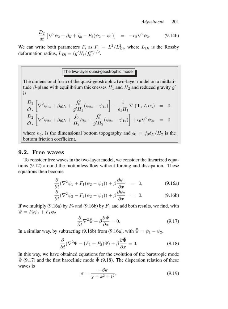
The two-layer quasi-geostrophic model
The dimensional form of the quasi-geostrophic two-layer model on a midlatitude β-plane with equilibrium thicknesses H 1 and H 2 and reduced gravity g ′
is
D 1
dt ∗
∇
2 ψ 1∗ + β 0 y ∗ +
f 2
0
g ′ H 1
(ψ 2∗ − ψ 1∗ )
−
1
ρ 1 H 1
∇.(T ∗ ∧ e 3 )=0 ,
D 2
dt ∗
∇
2 ψ 2∗ + β 0 y ∗ +
f 0
H 2
h b∗ −
f 2
0
g ′ H 2
(ψ 2∗ − ψ 1∗ )
+ ǫ 0 ∇
2 ψ 2∗ =0
where h b∗ is the dimensional bottom topography and ǫ 0 = f 0 δ E /H 2 is the
bottom friction coefficient.
9.2. Free waves
To consider free waves in the two-layer model, we consider the linearized equations (9.12) around the motionless flow without forcing and dissipation. These
equations then become
∂
∂t
(∇
2 ψ 1 + F 1 (ψ 2 − ψ 1 )) + β
∂ψ 1
∂x
=0 ,
(9.16a)
∂
∂t
(∇
2 ψ 2 − F 2 (ψ 2 − ψ 1 )) + β
∂ψ 2
∂x
=0 .
(9.16b)
If we multiply (9.16a) by F 2 and (9.16b) by F 1 and add both results, we find, with
˜
Ψ=F 2 ψ 1 + F 1 ψ 2
∂
∂t
∇
2 ˜
Ψ+β
∂ ˜
Ψ
∂x
=0.
(9.17)
In a similar way, by subtracting (9.16b) from (9.16a), with ¯
Ψ=ψ 1 − ψ 2 ,
∂
∂t
(∇
2 ¯
Ψ − (F 1 + F 2 ) ¯
Ψ) + β
∂ ¯
Ψ
∂x
=0.
(9.18)
In this way, we have obtained equations for the evolution of the barotropic mode
˜
Ψ (9.17) and the first baroclinic mode ¯
Ψ (9.18). The dispersion relation of these
waves is
σ =
−βk
χ + k 2 + l 2 ,
(9.19)
201
D 2
dt
∇
2 ψ 2 + βy +˜ η b − F 2 (ψ 2 − ψ 1 )
= −r 2 ∇
2 ψ 2 .
(9.14b)
We can write both parameters F i as F i = L 2 /L 2
Di , where L Di is the Rossby
deformation radius, L Di =(g ′ H i /f 2
0 ) 1/2 .
The two-layer quasi-geostrophic model
The dimensional form of the quasi-geostrophic two-layer model on a midlatitude β-plane with equilibrium thicknesses H 1 and H 2 and reduced gravity g ′
is
D 1
dt ∗
∇
2 ψ 1∗ + β 0 y ∗ +
f 2
0
g ′ H 1
(ψ 2∗ − ψ 1∗ )
−
1
ρ 1 H 1
∇.(T ∗ ∧ e 3 )=0 ,
D 2
dt ∗
∇
2 ψ 2∗ + β 0 y ∗ +
f 0
H 2
h b∗ −
f 2
0
g ′ H 2
(ψ 2∗ − ψ 1∗ )
+ ǫ 0 ∇
2 ψ 2∗ =0
where h b∗ is the dimensional bottom topography and ǫ 0 = f 0 δ E /H 2 is the
bottom friction coefficient.
9.2. Free waves
To consider free waves in the two-layer model, we consider the linearized equations (9.12) around the motionless flow without forcing and dissipation. These
equations then become
∂
∂t
(∇
2 ψ 1 + F 1 (ψ 2 − ψ 1 )) + β
∂ψ 1
∂x
=0 ,
(9.16a)
∂
∂t
(∇
2 ψ 2 − F 2 (ψ 2 − ψ 1 )) + β
∂ψ 2
∂x
=0 .
(9.16b)
If we multiply (9.16a) by F 2 and (9.16b) by F 1 and add both results, we find, with
˜
Ψ=F 2 ψ 1 + F 1 ψ 2
∂
∂t
∇
2 ˜
Ψ+β
∂ ˜
Ψ
∂x
=0.
(9.17)
In a similar way, by subtracting (9.16b) from (9.16a), with ¯
Ψ=ψ 1 − ψ 2 ,
∂
∂t
(∇
2 ¯
Ψ − (F 1 + F 2 ) ¯
Ψ) + β
∂ ¯
Ψ
∂x
=0.
(9.18)
In this way, we have obtained equations for the evolution of the barotropic mode
˜
Ψ (9.17) and the first baroclinic mode ¯
Ψ (9.18). The dispersion relation of these
waves is
σ =
−βk
χ + k 2 + l 2 ,
(9.19)