

Adjustment
199
where p I = ρ 1 gH 1 +p 0 is the equilibrium pressure at the equilibrium thermocline. Ex. 9.1
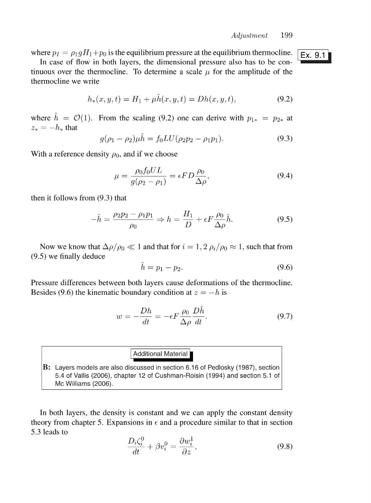
In case of flow in both layers, the dimensional pressure also has to be continuous over the thermocline. To determine a scale μ for the amplitude of the
thermocline we write
h ∗ (x, y, t)=H 1 + μ ˆ
h(x, y, t)=Dh(x, y, t),
(9.2)
where ˆ
h = O(1). From the scaling (9.2) one can derive with p 1∗ = p 2∗ at
z ∗ = −h ∗ that
g(ρ 1 − ρ 2 )μ ˆ
h = f 0 LU (ρ 2 p 2 − ρ 1 p 1 ).
(9.3)
With a reference density ρ 0 , and if we choose
μ =
ρ 0 f 0 UL
g(ρ 2 − ρ 1 )
= ǫF D
ρ 0
Δρ
,
(9.4)
then it follows from (9.3) that
− ˆ
h =
ρ 2 p 2 − ρ 1 p 1
ρ 0
⇒ h =
H 1
D
+ ǫF
ρ 0
Δρ
ˆ
h.
(9.5)
Now we know that Δρ/ρ 0 ≪ 1 and that for i =1, 2 ρ i /ρ 0 ≈ 1, such that from
(9.5) we finally deduce
ˆ
h = p 1 − p 2 .
(9.6)
Pressure differences between both layers cause deformations of the thermocline.
Besides (9.6) the kinematic boundary condition at z = −h is
w = −
Dh
dt
= −ǫF
ρ 0
Δρ
D ˆ
h
dt
.
(9.7)
Additional Material
B: Layers models are also discussed in section 6.16 of Pedlosky (1987), section
5.4 of Vallis (2006), chapter 12 of Cushman-Roisin (1994) and section 5.1 of
Mc Williams (2006).
In both layers, the density is constant and we can apply the constant density
theory from chapter 5. Expansions in ǫ and a procedure similar to that in section
5.3 leads to
D i ζ 0
i
dt
+ βv
0
i =
∂w 1
i
∂z
,
(9.8)
199
where p I = ρ 1 gH 1 +p 0 is the equilibrium pressure at the equilibrium thermocline. Ex. 9.1
In case of flow in both layers, the dimensional pressure also has to be continuous over the thermocline. To determine a scale μ for the amplitude of the
thermocline we write
h ∗ (x, y, t)=H 1 + μ ˆ
h(x, y, t)=Dh(x, y, t),
(9.2)
where ˆ
h = O(1). From the scaling (9.2) one can derive with p 1∗ = p 2∗ at
z ∗ = −h ∗ that
g(ρ 1 − ρ 2 )μ ˆ
h = f 0 LU (ρ 2 p 2 − ρ 1 p 1 ).
(9.3)
With a reference density ρ 0 , and if we choose
μ =
ρ 0 f 0 UL
g(ρ 2 − ρ 1 )
= ǫF D
ρ 0
Δρ
,
(9.4)
then it follows from (9.3) that
− ˆ
h =
ρ 2 p 2 − ρ 1 p 1
ρ 0
⇒ h =
H 1
D
+ ǫF
ρ 0
Δρ
ˆ
h.
(9.5)
Now we know that Δρ/ρ 0 ≪ 1 and that for i =1, 2 ρ i /ρ 0 ≈ 1, such that from
(9.5) we finally deduce
ˆ
h = p 1 − p 2 .
(9.6)
Pressure differences between both layers cause deformations of the thermocline.
Besides (9.6) the kinematic boundary condition at z = −h is
w = −
Dh
dt
= −ǫF
ρ 0
Δρ
D ˆ
h
dt
.
(9.7)
Additional Material
B: Layers models are also discussed in section 6.16 of Pedlosky (1987), section
5.4 of Vallis (2006), chapter 12 of Cushman-Roisin (1994) and section 5.1 of
Mc Williams (2006).
In both layers, the density is constant and we can apply the constant density
theory from chapter 5. Expansions in ǫ and a procedure similar to that in section
5.3 leads to
D i ζ 0
i
dt
+ βv
0
i =
∂w 1
i
∂z
,
(9.8)