

198
DYNAMICAL OCEANOGRAPHY
After the discussion on the free waves in the stratified and constant density case, we can now tackle the adjustment problem already mentioned
in chapter 7. How does the time-dependent flow from a motionless state
settle into a steady ocean circulation once a wind stress is forcing it? We
therefore consider in this chapter a basin stratified motionless ocean that
is suddenly forced by a wind-stress field. For the stratified case, we will
restrict ourselves to the analysis of the two-layer model that will be derived in section 9.1; its free waves will be presented in section 9.2. In the
constant density case we know that for t →∞, a Sverdrup balance with a
western boundary current will appear. It will turn out that the adjustment
can be studied simultaneously in the constant density and two-layer case
(section 9.3)
9.1. The quasi-geostrophic two-layer model
As the ocean stratification can be imagined to be build up of layers which are
advected without much mixing, layer models have been frequently used as a simplification of the continuous stratified model. In each layer, the density is assumed
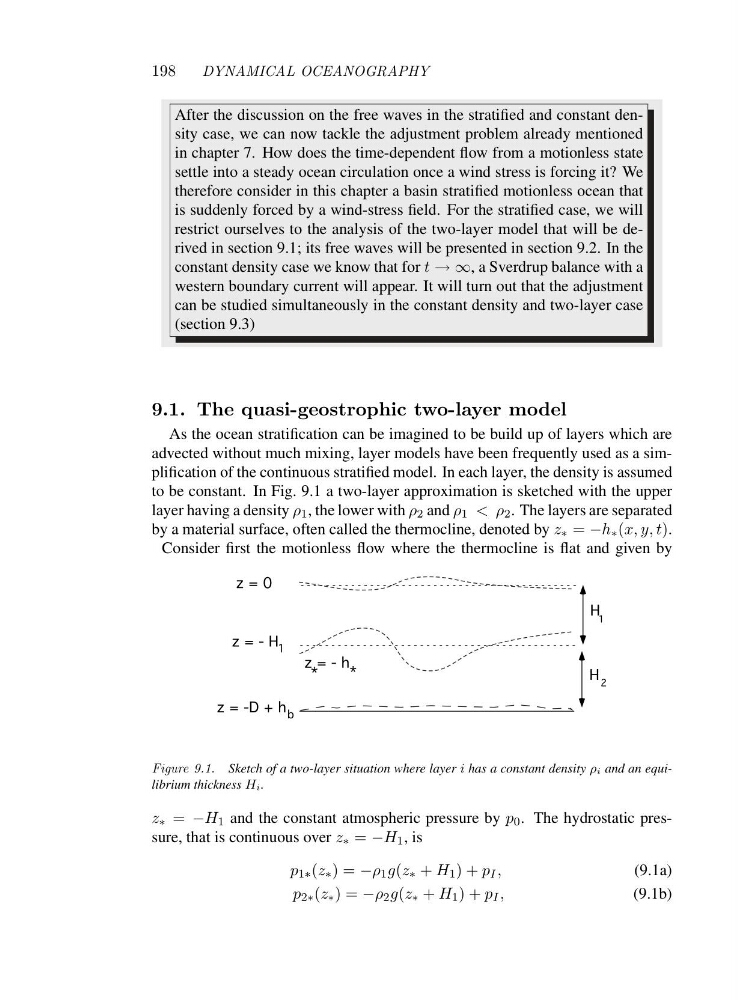
to be constant. In Fig. 9.1 a two-layer approximation is sketched with the upper
layer having a density ρ 1 , the lower with ρ 2 and ρ 1 <ρ 2 . The layers are separated
by a material surface, often called the thermocline, denoted by z ∗ = −h ∗ (x, y, t).
Consider first the motionless flow where the thermocline is flat and given by
H 1
H 2
z = - h
*
*
z = 0
z = -D + h b
z = - H 1
Figure 9.1. Sketch of a two-layer situation where layer i has a constant density ρi and an equilibrium thickness Hi.
z ∗ = −H 1 and the constant atmospheric pressure by p 0 . The hydrostatic pressure, that is continuous over z ∗ = −H 1 ,is
p 1∗ (z ∗ )=−ρ 1 g(z ∗ + H 1 )+p I ,
(9.1a)
p 2∗ (z ∗ )=−ρ 2 g(z ∗ + H 1 )+p I ,
(9.1b)
DYNAMICAL OCEANOGRAPHY
After the discussion on the free waves in the stratified and constant density case, we can now tackle the adjustment problem already mentioned
in chapter 7. How does the time-dependent flow from a motionless state
settle into a steady ocean circulation once a wind stress is forcing it? We
therefore consider in this chapter a basin stratified motionless ocean that
is suddenly forced by a wind-stress field. For the stratified case, we will
restrict ourselves to the analysis of the two-layer model that will be derived in section 9.1; its free waves will be presented in section 9.2. In the
constant density case we know that for t →∞, a Sverdrup balance with a
western boundary current will appear. It will turn out that the adjustment
can be studied simultaneously in the constant density and two-layer case
(section 9.3)
9.1. The quasi-geostrophic two-layer model
As the ocean stratification can be imagined to be build up of layers which are
advected without much mixing, layer models have been frequently used as a simplification of the continuous stratified model. In each layer, the density is assumed
to be constant. In Fig. 9.1 a two-layer approximation is sketched with the upper
layer having a density ρ 1 , the lower with ρ 2 and ρ 1 <ρ 2 . The layers are separated
by a material surface, often called the thermocline, denoted by z ∗ = −h ∗ (x, y, t).
Consider first the motionless flow where the thermocline is flat and given by
H 1
H 2
z = - h
*
*
z = 0
z = -D + h b
z = - H 1
Figure 9.1. Sketch of a two-layer situation where layer i has a constant density ρi and an equilibrium thickness Hi.
z ∗ = −H 1 and the constant atmospheric pressure by p 0 . The hydrostatic pressure, that is continuous over z ∗ = −H 1 ,is
p 1∗ (z ∗ )=−ρ 1 g(z ∗ + H 1 )+p I ,
(9.1a)
p 2∗ (z ∗ )=−ρ 2 g(z ∗ + H 1 )+p I ,
(9.1b)