

158
DYNAMICAL OCEANOGRAPHY
If η is determined, then it follows that ˜
h = η and the velocities ˜
u and ˜
v follow
by differentiating (7.3a-b) with respect to t with the result
(
∂ 2
∂t 2 + f
2 )˜ u = −g
∂ 2˜ h
∂x∂t
+ f
∂ ˜
h
∂y
,
(7.10a)
(
∂ 2
∂t 2 + f
2 )˜ v = −g
∂ 2˜ h
∂y∂t
− f
∂ ˜
h
∂x
.
(7.10b)
The equations above describe the evolution of small amplitude perturbations on
the motionless solution. In the next sections, we will consider specific geometrical
situations and determine the free wave solutions in these cases.
7.2. Free waves: H 0 constant
In the case where H 0 is constant, we introduce C 2
0 = gH 0 and (7.9) reduces to
∂
∂t
(
∂ 2
∂t 2 + f
2 )η − C
2
0 ∇
2
H η
=0,
(7.11)
where ∇ 2
H = ∂ 2 /∂x 2 + ∂ 2 /∂y 2 is the horizontal Laplace operator.
7.2.1. Unbounded domain
When the domain is horizontally unbounded, there exist free wave solutions of
(7.11) with the representation
η(x, y, t)=η 0 e
i(kx+ly−σt) ,
(7.12)
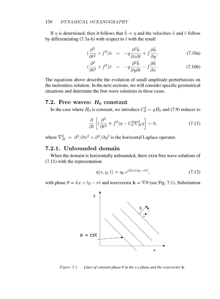
with phase θ = kx + ly − σt and wavevector k = ∇θ (see Fig. 7.1). Substitution
θ = cst
k
l
k
x
y
Figure 7.1. Lines of constant phase θ in the x-y plane and the wavevector k.
DYNAMICAL OCEANOGRAPHY
If η is determined, then it follows that ˜
h = η and the velocities ˜
u and ˜
v follow
by differentiating (7.3a-b) with respect to t with the result
(
∂ 2
∂t 2 + f
2 )˜ u = −g
∂ 2˜ h
∂x∂t
+ f
∂ ˜
h
∂y
,
(7.10a)
(
∂ 2
∂t 2 + f
2 )˜ v = −g
∂ 2˜ h
∂y∂t
− f
∂ ˜
h
∂x
.
(7.10b)
The equations above describe the evolution of small amplitude perturbations on
the motionless solution. In the next sections, we will consider specific geometrical
situations and determine the free wave solutions in these cases.
7.2. Free waves: H 0 constant
In the case where H 0 is constant, we introduce C 2
0 = gH 0 and (7.9) reduces to
∂
∂t
(
∂ 2
∂t 2 + f
2 )η − C
2
0 ∇
2
H η
=0,
(7.11)
where ∇ 2
H = ∂ 2 /∂x 2 + ∂ 2 /∂y 2 is the horizontal Laplace operator.
7.2.1. Unbounded domain
When the domain is horizontally unbounded, there exist free wave solutions of
(7.11) with the representation
η(x, y, t)=η 0 e
i(kx+ly−σt) ,
(7.12)
with phase θ = kx + ly − σt and wavevector k = ∇θ (see Fig. 7.1). Substitution
θ = cst
k
l
k
x
y
Figure 7.1. Lines of constant phase θ in the x-y plane and the wavevector k.