

144
DYNAMICAL OCEANOGRAPHY
will show damped oscillatory behavior when u 0 (x W ,y) > 0 and cannot satisfy
the matching condition (6.78). Hence, a necessary condition for the existence of
an inertial boundary layer is
u
0 (x W ,y) < 0.
(6.80)
In Fig. 6.6, we see that south of y 0 , where u 0 < 0, there can be an inertial boundary layer. For y>y 0 , a pure inertial layer cannot occur and the excess of relative
vorticity has to be dissipated through friction.
Additional Material
B: A less mathematical approach to the Sverdrup balance and western boundary
layers can be found in chapter 8 of Cushman-Roisin (1994).
D: Having understood the material so far, extensions within reach are chapter 5
of Pedlosky (1987), where much more details are provided of the theory of
the homogeneous wind-driven circulation, and chapter 14 (sections 14.1 to
14.6) of Vallis (2006) where for example topographic effects are discussed.
6.4. Highly nonlinear flows
-1.5
-1
-0.5
0
0.5
1
1.5
0
0.2
0.4
0.6
0.8
1
single - gyre
double - gyre
y/L
τ τ
τ
τ
x x x
x
/ / /
/τ τ
τ
τ 0 0
0
0
0.0
1.0
0.5
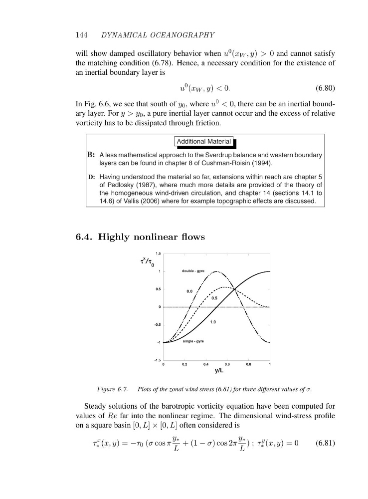
Figure 6.7. Plots of the zonal wind stress (6.81) for three different values of σ.
Steady solutions of the barotropic vorticity equation have been computed for
values of Re far into the nonlinear regime. The dimensional wind-stress profile
on a square basin [0,L] × [0,L] often considered is
τ
x
∗ (x, y)=−τ 0 (σ cos π
y ∗
L
+(1− σ)cos2π
y ∗
L
); τ
y
∗ (x, y)=0
(6.81)
DYNAMICAL OCEANOGRAPHY
will show damped oscillatory behavior when u 0 (x W ,y) > 0 and cannot satisfy
the matching condition (6.78). Hence, a necessary condition for the existence of
an inertial boundary layer is
u
0 (x W ,y) < 0.
(6.80)
In Fig. 6.6, we see that south of y 0 , where u 0 < 0, there can be an inertial boundary layer. For y>y 0 , a pure inertial layer cannot occur and the excess of relative
vorticity has to be dissipated through friction.
Additional Material
B: A less mathematical approach to the Sverdrup balance and western boundary
layers can be found in chapter 8 of Cushman-Roisin (1994).
D: Having understood the material so far, extensions within reach are chapter 5
of Pedlosky (1987), where much more details are provided of the theory of
the homogeneous wind-driven circulation, and chapter 14 (sections 14.1 to
14.6) of Vallis (2006) where for example topographic effects are discussed.
6.4. Highly nonlinear flows
-1.5
-1
-0.5
0
0.5
1
1.5
0
0.2
0.4
0.6
0.8
1
single - gyre
double - gyre
y/L
τ τ
τ
τ
x x x
x
/ / /
/τ τ
τ
τ 0 0
0
0
0.0
1.0
0.5
Figure 6.7. Plots of the zonal wind stress (6.81) for three different values of σ.
Steady solutions of the barotropic vorticity equation have been computed for
values of Re far into the nonlinear regime. The dimensional wind-stress profile
on a square basin [0,L] × [0,L] often considered is
τ
x
∗ (x, y)=−τ 0 (σ cos π
y ∗
L
+(1− σ)cos2π
y ∗
L
); τ
y
∗ (x, y)=0
(6.81)