

Western intensification
143
Equation (6.76) expresses that the quasi-geostrophic potential vorticity (cf. section 5.3) is constant along streamlines.
y
1
y
2
U < 0
U > 0
y
0
δ I
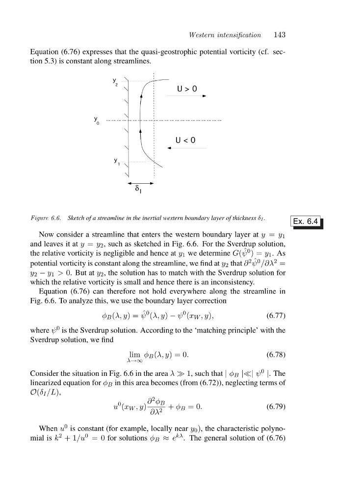
Figure 6.6. Sketch of a streamline in the inertial western boundary layer of thickness δI .
Ex. 6.4
Now consider a streamline that enters the western boundary layer at y = y 1
and leaves it at y = y 2 , such as sketched in Fig. 6.6. For the Sverdrup solution,
the relative vorticity is negligible and hence at y 1 we determine G( ˆ
ψ 0 )=y 1 .A s
potential vorticity is constant along the streamline, we find at y 2 that ∂ 2 ˆ
ψ 0 /∂λ 2 =
y 2 − y 1 > 0.B u ta ty 2 , the solution has to match with the Sverdrup solution for
which the relative vorticity is small and hence there is an inconsistency.
Equation (6.76) can therefore not hold everywhere along the streamline in
Fig. 6.6. To analyze this, we use the boundary layer correction
φ B (λ, y)= ˆ
ψ
0 (λ, y) − ψ
0 (x W ,y),
(6.77)
where ψ 0 is the Sverdrup solution. According to the ‘matching principle’ with the
Sverdrup solution, we find
lim
λ→∞
φ B (λ, y)=0.
(6.78)
Consider the situation in Fig. 6.6 in the area λ ≫ 1, such that | φ B |≪| ψ 0 |.T h e
linearized equation for φ B in this area becomes (from (6.72)), neglecting terms of
O(δ I /L),
u
0 (x W ,y)
∂ 2 φ B
∂λ 2 + φ B =0.
(6.79)
When u 0 is constant (for example, locally near y 0 ), the characteristic polynomial is k 2 +1/u 0 =0for solutions φ B ≈ e kλ . The general solution of (6.76)
143
Equation (6.76) expresses that the quasi-geostrophic potential vorticity (cf. section 5.3) is constant along streamlines.
y
1
y
2
U < 0
U > 0
y
0
δ I
Figure 6.6. Sketch of a streamline in the inertial western boundary layer of thickness δI .
Ex. 6.4
Now consider a streamline that enters the western boundary layer at y = y 1
and leaves it at y = y 2 , such as sketched in Fig. 6.6. For the Sverdrup solution,
the relative vorticity is negligible and hence at y 1 we determine G( ˆ
ψ 0 )=y 1 .A s
potential vorticity is constant along the streamline, we find at y 2 that ∂ 2 ˆ
ψ 0 /∂λ 2 =
y 2 − y 1 > 0.B u ta ty 2 , the solution has to match with the Sverdrup solution for
which the relative vorticity is small and hence there is an inconsistency.
Equation (6.76) can therefore not hold everywhere along the streamline in
Fig. 6.6. To analyze this, we use the boundary layer correction
φ B (λ, y)= ˆ
ψ
0 (λ, y) − ψ
0 (x W ,y),
(6.77)
where ψ 0 is the Sverdrup solution. According to the ‘matching principle’ with the
Sverdrup solution, we find
lim
λ→∞
φ B (λ, y)=0.
(6.78)
Consider the situation in Fig. 6.6 in the area λ ≫ 1, such that | φ B |≪| ψ 0 |.T h e
linearized equation for φ B in this area becomes (from (6.72)), neglecting terms of
O(δ I /L),
u
0 (x W ,y)
∂ 2 φ B
∂λ 2 + φ B =0.
(6.79)
When u 0 is constant (for example, locally near y 0 ), the characteristic polynomial is k 2 +1/u 0 =0for solutions φ B ≈ e kλ . The general solution of (6.76)