

142
DYNAMICAL OCEANOGRAPHY
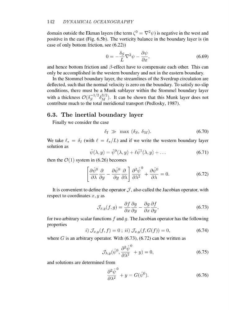
domain outside the Ekman layers (the term ζ 0 = ∇ 2 ψ) is negative in the west and
positive in the east (Fig. 6.5b). The vorticity balance in the boundary layer is (in
case of only bottom friction, see (6.22))
0=−
δ S
L
∇
2 ψ −
∂ψ
∂x
,
(6.69)
and hence bottom friction and β-effect have to compensate each other. This can
only be accomplished in the western boundary and not in the eastern boundary.
In the Stommel boundary layer, the streamlines of the Sverdrup circulation are
deflected, such that the normal velocity is zero on the boundary. To satisfy no-slip
conditions, there must be a Munk sublayer within the Stommel boundary layer
with a thickness O(δ
−1/2
S
δ
3/2
M ). It can be shown that this Munk layer does not
contribute much to the total meridional transport (Pedlosky, 1987).
6.3. The inertial boundary layer
Finally we consider the case
δ I ≫ max (δ S ,δ M ).
(6.70)
We take ℓ ∗ = δ I (with ℓ = ℓ ∗ /L) and if we write the western boundary layer
solution as
ˆ
ψ(λ, y)= ˆ
ψ
0 (λ, y)+ℓ ˆ
ψ
1 (λ, y)+...
(6.71)
then the O(1) system in (6.26) becomes
∂ ˆ
ψ 0
∂λ
∂
∂y
−
∂ ˆ
ψ 0
∂y
∂
∂λ
∂ 2 ˆ
ψ
∂λ 2
0
+
∂ ˆ
ψ 0
∂λ
=0.
(6.72)
It is convenient to define the operator J , also called the Jacobian operator, with
respect to coordinates x, y as
J x,y (f, g)=
∂f
∂x
∂g
∂y
−
∂g
∂x
∂f
∂y
,
(6.73)
for two arbitrary scalar functions f and g. The Jacobian operator has the following
properties
i) J x,y (f, f)=0; ii) J x,y (f, G(f )) = 0,
(6.74)
where G is an arbitrary operator. With (6.73), (6.72) can be written as
J λ,y ( ˆ
ψ
0 ,
∂ 2 ˆ
ψ
∂λ 2
0
+ y)=0,
(6.75)
and solutions are determined from
∂ 2 ˆ
ψ
∂λ 2
0
+ y = G( ˆ
ψ
0 ).
(6.76)
DYNAMICAL OCEANOGRAPHY
domain outside the Ekman layers (the term ζ 0 = ∇ 2 ψ) is negative in the west and
positive in the east (Fig. 6.5b). The vorticity balance in the boundary layer is (in
case of only bottom friction, see (6.22))
0=−
δ S
L
∇
2 ψ −
∂ψ
∂x
,
(6.69)
and hence bottom friction and β-effect have to compensate each other. This can
only be accomplished in the western boundary and not in the eastern boundary.
In the Stommel boundary layer, the streamlines of the Sverdrup circulation are
deflected, such that the normal velocity is zero on the boundary. To satisfy no-slip
conditions, there must be a Munk sublayer within the Stommel boundary layer
with a thickness O(δ
−1/2
S
δ
3/2
M ). It can be shown that this Munk layer does not
contribute much to the total meridional transport (Pedlosky, 1987).
6.3. The inertial boundary layer
Finally we consider the case
δ I ≫ max (δ S ,δ M ).
(6.70)
We take ℓ ∗ = δ I (with ℓ = ℓ ∗ /L) and if we write the western boundary layer
solution as
ˆ
ψ(λ, y)= ˆ
ψ
0 (λ, y)+ℓ ˆ
ψ
1 (λ, y)+...
(6.71)
then the O(1) system in (6.26) becomes
∂ ˆ
ψ 0
∂λ
∂
∂y
−
∂ ˆ
ψ 0
∂y
∂
∂λ
∂ 2 ˆ
ψ
∂λ 2
0
+
∂ ˆ
ψ 0
∂λ
=0.
(6.72)
It is convenient to define the operator J , also called the Jacobian operator, with
respect to coordinates x, y as
J x,y (f, g)=
∂f
∂x
∂g
∂y
−
∂g
∂x
∂f
∂y
,
(6.73)
for two arbitrary scalar functions f and g. The Jacobian operator has the following
properties
i) J x,y (f, f)=0; ii) J x,y (f, G(f )) = 0,
(6.74)
where G is an arbitrary operator. With (6.73), (6.72) can be written as
J λ,y ( ˆ
ψ
0 ,
∂ 2 ˆ
ψ
∂λ 2
0
+ y)=0,
(6.75)
and solutions are determined from
∂ 2 ˆ
ψ
∂λ 2
0
+ y = G( ˆ
ψ
0 ).
(6.76)