

118
DYNAMICAL OCEANOGRAPHY
5.4. The barotropic vorticity equation
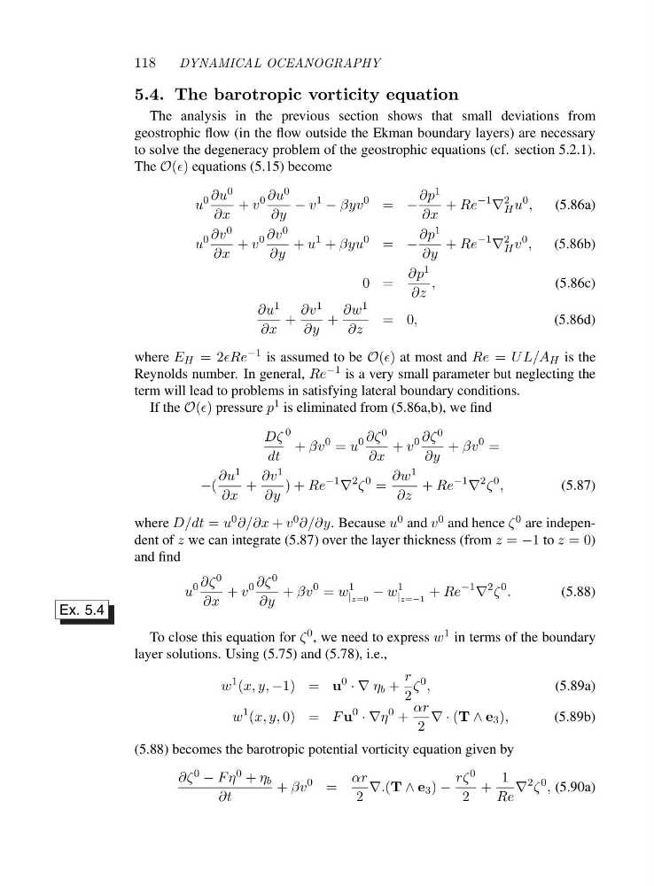
The analysis in the previous section shows that small deviations from
geostrophic flow (in the flow outside the Ekman boundary layers) are necessary
to solve the degeneracy problem of the geostrophic equations (cf. section 5.2.1).
The O(ǫ) equations (5.15) become
u
0 ∂u 0
∂x
+ v
0 ∂u 0
∂y
− v
1 − βyv
0 = −
∂p 1
∂x
+ Re
−1 ∇
2
H u
0 ,
(5.86a)
u
0 ∂v 0
∂x
+ v
0 ∂v 0
∂y
+ u
1 + βyu
0 = −
∂p 1
∂y
+ Re
−1 ∇
2
H v
0 ,
(5.86b)
0=
∂p 1
∂z
,
(5.86c)
∂u 1
∂x
+
∂v 1
∂y
+
∂w 1
∂z
=0 ,
(5.86d)
where E H =2 ǫRe −1 is assumed to be O(ǫ) at most and Re = UL/A H is the
Reynolds number. In general, Re −1 is a very small parameter but neglecting the
term will lead to problems in satisfying lateral boundary conditions.
If the O(ǫ) pressure p 1 is eliminated from (5.86a,b), we find
Dζ
dt
0
+ βv
0 = u
0 ∂ζ 0
∂x
+ v
0 ∂ζ 0
∂y
+ βv
0 =
−(
∂u 1
∂x
+
∂v 1
∂y
)+Re
−1 ∇
2 ζ
0 =
∂w 1
∂z
+ Re
−1 ∇
2 ζ
0 ,
(5.87)
where D/dt = u 0 ∂/∂x + v 0 ∂/∂y. Because u 0 and v 0 and hence ζ 0 are independent of z we can integrate (5.87) over the layer thickness (from z = −1 to z =0)
and find
Ex. 5.4
u
0 ∂ζ 0
∂x
+ v
0 ∂ζ 0
∂y
+ βv
0 = w
1
|z=0 − w
1
|z=−1 + Re
−1 ∇
2 ζ
0 .
(5.88)
To close this equation for ζ 0 , we need to express w 1 in terms of the boundary
layer solutions. Using (5.75) and (5.78), i.e.,
w
1 (x, y, −1) = u
0 ·∇η b +
r
2
ζ
0 ,
(5.89a)
w
1 (x, y, 0) = F u
0 ·∇η
0 +
αr
2
∇·(T ∧ e 3 ),
(5.89b)
(5.88) becomes the barotropic potential vorticity equation given by
∂ζ 0 − Fη 0 + η b
∂t
+ βv
0 =
αr
2
∇.(T ∧ e 3 ) −
rζ 0
2
+
1
Re
∇
2 ζ
0 , (5.90a)
DYNAMICAL OCEANOGRAPHY
5.4. The barotropic vorticity equation
The analysis in the previous section shows that small deviations from
geostrophic flow (in the flow outside the Ekman boundary layers) are necessary
to solve the degeneracy problem of the geostrophic equations (cf. section 5.2.1).
The O(ǫ) equations (5.15) become
u
0 ∂u 0
∂x
+ v
0 ∂u 0
∂y
− v
1 − βyv
0 = −
∂p 1
∂x
+ Re
−1 ∇
2
H u
0 ,
(5.86a)
u
0 ∂v 0
∂x
+ v
0 ∂v 0
∂y
+ u
1 + βyu
0 = −
∂p 1
∂y
+ Re
−1 ∇
2
H v
0 ,
(5.86b)
0=
∂p 1
∂z
,
(5.86c)
∂u 1
∂x
+
∂v 1
∂y
+
∂w 1
∂z
=0 ,
(5.86d)
where E H =2 ǫRe −1 is assumed to be O(ǫ) at most and Re = UL/A H is the
Reynolds number. In general, Re −1 is a very small parameter but neglecting the
term will lead to problems in satisfying lateral boundary conditions.
If the O(ǫ) pressure p 1 is eliminated from (5.86a,b), we find
Dζ
dt
0
+ βv
0 = u
0 ∂ζ 0
∂x
+ v
0 ∂ζ 0
∂y
+ βv
0 =
−(
∂u 1
∂x
+
∂v 1
∂y
)+Re
−1 ∇
2 ζ
0 =
∂w 1
∂z
+ Re
−1 ∇
2 ζ
0 ,
(5.87)
where D/dt = u 0 ∂/∂x + v 0 ∂/∂y. Because u 0 and v 0 and hence ζ 0 are independent of z we can integrate (5.87) over the layer thickness (from z = −1 to z =0)
and find
Ex. 5.4
u
0 ∂ζ 0
∂x
+ v
0 ∂ζ 0
∂y
+ βv
0 = w
1
|z=0 − w
1
|z=−1 + Re
−1 ∇
2 ζ
0 .
(5.88)
To close this equation for ζ 0 , we need to express w 1 in terms of the boundary
layer solutions. Using (5.75) and (5.78), i.e.,
w
1 (x, y, −1) = u
0 ·∇η b +
r
2
ζ
0 ,
(5.89a)
w
1 (x, y, 0) = F u
0 ·∇η
0 +
αr
2
∇·(T ∧ e 3 ),
(5.89b)
(5.88) becomes the barotropic potential vorticity equation given by
∂ζ 0 − Fη 0 + η b
∂t
+ βv
0 =
αr
2
∇.(T ∧ e 3 ) −
rζ 0
2
+
1
Re
∇
2 ζ
0 , (5.90a)