

Wind-driven circulation
117
Surface Ekman layer
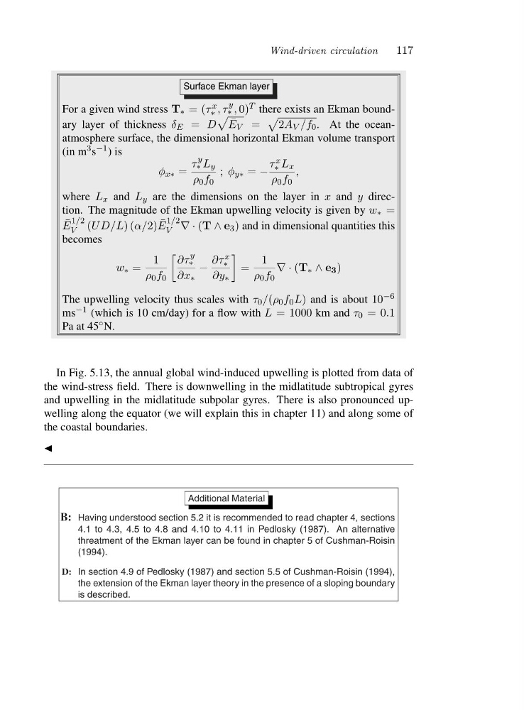
For a given wind stress T ∗ =( τ x
∗ ,τ
y
∗ , 0) T there exists an Ekman boundary layer of thickness δ E = D
¯
E V =
2A V /f 0 . At the oceanatmosphere surface, the dimensional horizontal Ekman volume transport
(in m 3 s −1 )is
φ x∗ =
τ
y
∗ L y
ρ 0 f 0
; φ y∗ = −
τ x
∗ L x
ρ 0 f 0
,
where L x and L y are the dimensions on the layer in x and y direction. The magnitude of the Ekman upwelling velocity is given by w ∗ =
¯
E
1/2
V (UD/L)(α/2) ¯
E
1/2
V ∇·(T ∧ e 3 ) and in dimensional quantities this
becomes
w ∗ =
1
ρ 0 f 0
∂τ
y
∗
∂x ∗
−
∂τ x
∗
∂y ∗
=
1
ρ 0 f 0
∇·(T ∗ ∧ e 3 )
The upwelling velocity thus scales with τ 0 /(ρ 0 f 0 L) and is about 10 −6
ms −1 (which is 10 cm/day) for a flow with L = 1000 km and τ 0 =0 .1
Pa at 45 ◦ N.
In Fig. 5.13, the annual global wind-induced upwelling is plotted from data of
the wind-stress field. There is downwelling in the midlatitude subtropical gyres
and upwelling in the midlatitude subpolar gyres. There is also pronounced upwelling along the equator (we will explain this in chapter 11) and along some of
the coastal boundaries.
◭
Additional Material
B: Having understood section 5.2 it is recommended to read chapter 4, sections
4.1 to 4.3, 4.5 to 4.8 and 4.10 to 4.11 in Pedlosky (1987). An alternative
threatment of the Ekman layer can be found in chapter 5 of Cushman-Roisin
(1994).
D: In section 4.9 of Pedlosky (1987) and section 5.5 of Cushman-Roisin (1994),
the extension of the Ekman layer theory in the presence of a sloping boundary
is described.
117
Surface Ekman layer
For a given wind stress T ∗ =( τ x
∗ ,τ
y
∗ , 0) T there exists an Ekman boundary layer of thickness δ E = D
¯
E V =
2A V /f 0 . At the oceanatmosphere surface, the dimensional horizontal Ekman volume transport
(in m 3 s −1 )is
φ x∗ =
τ
y
∗ L y
ρ 0 f 0
; φ y∗ = −
τ x
∗ L x
ρ 0 f 0
,
where L x and L y are the dimensions on the layer in x and y direction. The magnitude of the Ekman upwelling velocity is given by w ∗ =
¯
E
1/2
V (UD/L)(α/2) ¯
E
1/2
V ∇·(T ∧ e 3 ) and in dimensional quantities this
becomes
w ∗ =
1
ρ 0 f 0
∂τ
y
∗
∂x ∗
−
∂τ x
∗
∂y ∗
=
1
ρ 0 f 0
∇·(T ∗ ∧ e 3 )
The upwelling velocity thus scales with τ 0 /(ρ 0 f 0 L) and is about 10 −6
ms −1 (which is 10 cm/day) for a flow with L = 1000 km and τ 0 =0 .1
Pa at 45 ◦ N.
In Fig. 5.13, the annual global wind-induced upwelling is plotted from data of
the wind-stress field. There is downwelling in the midlatitude subtropical gyres
and upwelling in the midlatitude subpolar gyres. There is also pronounced upwelling along the equator (we will explain this in chapter 11) and along some of
the coastal boundaries.
◭
Additional Material
B: Having understood section 5.2 it is recommended to read chapter 4, sections
4.1 to 4.3, 4.5 to 4.8 and 4.10 to 4.11 in Pedlosky (1987). An alternative
threatment of the Ekman layer can be found in chapter 5 of Cushman-Roisin
(1994).
D: In section 4.9 of Pedlosky (1987) and section 5.5 of Cushman-Roisin (1994),
the extension of the Ekman layer theory in the presence of a sloping boundary
is described.