

110
DYNAMICAL OCEANOGRAPHY
L y
L x
δ
φφ
E
y
x
Ekman layer
Geostrophic regime
z = - D
z
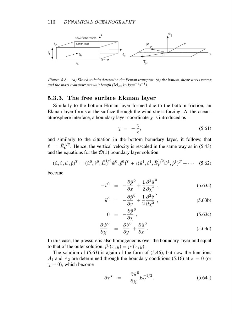
Figure 5.8. (a) Sketch to help determine the Ekman transport. (b) the bottom shear stress vector
and the mass transport per unit length (ME∗in kgm
−1 s
−1 ).
5.3.3. The free surface Ekman layer
Similarly to the bottom Ekman layer formed due to the bottom friction, an
Ekman layer forms at the surface through the wind-stress forcing. At the oceanatmosphere interface, a boundary layer coordinate χ is introduced as
χ = −
z
ℓ
,
(5.61)
and similarly to the situation in the bottom boundary layer, it follows that
ℓ = ¯
E
1/2
V . Hence, the vertical velocity is rescaled in the same way as in (5.43)
and the equations for the O(1) boundary layer solution
(ˆ u, ˆ
v, ˆ
w, ˆ
p)
T =(ˆ u
0 , ˆ
v
0 , ¯
E
1/2
V ˆ
w
0 , ˆ
p
0 )
T + ǫ(ˆ u
1 , ˆ
v
1 , ¯
E
1/2
V ˆ
w
1 , ˆ
p
1 )
T + ··· (5.62)
become
−ˆ v
0 = −
∂ ˆ
p
∂x
0
+
1
2
∂ 2 ˆ
u
∂χ 2
0
,
(5.63a)
˜
u
0 = −
∂ ˆ
p
∂y
0
+
1
2
∂ 2 ˆ
v
∂χ 2
0
,
(5.63b)
0=−
∂ ˆ
p
∂χ
0
,
(5.63c)
∂ ˆ
w
∂χ
0
=
∂ˆ v
∂y
0
+
∂ ˆ
u
∂x
0
.
(5.63d)
In this case, the pressure is also homogeneous over the boundary layer and equal
to that of the outer solution, ˆ
p 0 (x, y)=p 0 (x, y).
The solution of (5.63) is again of the form of (5.46), but now the functions
A 1 and A 2 are determined through the boundary conditions (5.16) at z =0(or
χ =0), which become
ˆ
ατ
x = −
∂ ˆ
u
∂χ
0
¯
E
−1/2
V
,
(5.64a)
DYNAMICAL OCEANOGRAPHY
L y
L x
δ
φφ
E
y
x
Ekman layer
Geostrophic regime
z = - D
z
Figure 5.8. (a) Sketch to help determine the Ekman transport. (b) the bottom shear stress vector
and the mass transport per unit length (ME∗in kgm
−1 s
−1 ).
5.3.3. The free surface Ekman layer
Similarly to the bottom Ekman layer formed due to the bottom friction, an
Ekman layer forms at the surface through the wind-stress forcing. At the oceanatmosphere interface, a boundary layer coordinate χ is introduced as
χ = −
z
ℓ
,
(5.61)
and similarly to the situation in the bottom boundary layer, it follows that
ℓ = ¯
E
1/2
V . Hence, the vertical velocity is rescaled in the same way as in (5.43)
and the equations for the O(1) boundary layer solution
(ˆ u, ˆ
v, ˆ
w, ˆ
p)
T =(ˆ u
0 , ˆ
v
0 , ¯
E
1/2
V ˆ
w
0 , ˆ
p
0 )
T + ǫ(ˆ u
1 , ˆ
v
1 , ¯
E
1/2
V ˆ
w
1 , ˆ
p
1 )
T + ··· (5.62)
become
−ˆ v
0 = −
∂ ˆ
p
∂x
0
+
1
2
∂ 2 ˆ
u
∂χ 2
0
,
(5.63a)
˜
u
0 = −
∂ ˆ
p
∂y
0
+
1
2
∂ 2 ˆ
v
∂χ 2
0
,
(5.63b)
0=−
∂ ˆ
p
∂χ
0
,
(5.63c)
∂ ˆ
w
∂χ
0
=
∂ˆ v
∂y
0
+
∂ ˆ
u
∂x
0
.
(5.63d)
In this case, the pressure is also homogeneous over the boundary layer and equal
to that of the outer solution, ˆ
p 0 (x, y)=p 0 (x, y).
The solution of (5.63) is again of the form of (5.46), but now the functions
A 1 and A 2 are determined through the boundary conditions (5.16) at z =0(or
χ =0), which become
ˆ
ατ
x = −
∂ ˆ
u
∂χ
0
¯
E
−1/2
V
,
(5.64a)